Amari's Natural Gradient

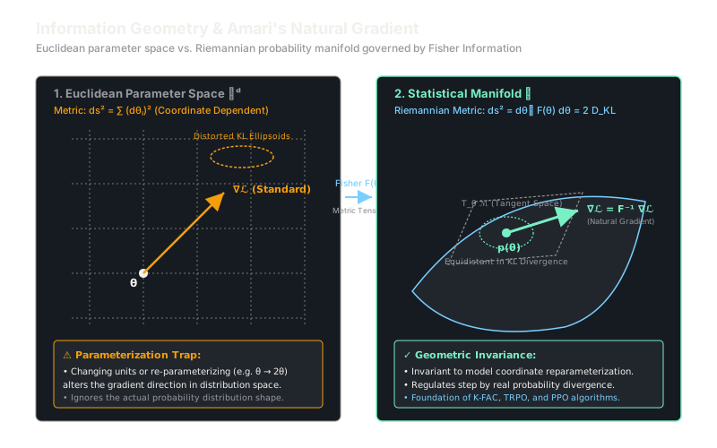
Natural gradient descent measures distance between probability distributions rather than arbitrary parameter coordinates, following steepest descent on a Riemannian manifold.

Euclidean gradient steps depend on arbitrary parameterization and distort distribution shifts, whereas natural gradient steps follow the intrinsic Riemannian metric defined by Fisher information.

Why Does This Exist?

Standard gradient descent defines "steepest descent" using the standard Euclidean distance metric in coordinate space: $\|\Delta \mathbf{\theta}\|^2 = \sum_i (\Delta \theta_i)^2$ . When parameters represent physical coordinates on a flat plane, this metric makes total sense.

In modern probabilistic machine learning — including neural networks with softmax classification, policy gradients in reinforcement learning, and variational autoencoders — parameters $\mathbf{\theta}$ do not represent physical locations. They define a probability distribution $p(\mathbf{x}; \mathbf{\theta})$ .

Euclidean parameter distance has virtually no relationship with the actual change in the underlying probability distribution. Consider a Gaussian distribution $\mathcal{N}(\mu, \sigma^2)$ :

Shifting mean $\mu$ by $0.1$ when $\sigma^2 = 100$ barely nudges the distribution; the Kullback-Leibler (KL) divergence is negligible.
Shifting $\mu$ by that same $0.1$ when $\sigma^2 = 0.001$ produces two non-overlapping spikes; the KL divergence explodes.

Standard gradient descent takes identical step sizes in both scenarios because it is blinded by coordinate Euclidean distance. Even worse, if you change units (e.g., scaling weights or swapping to polar coordinates), the standard gradient changes direction entirely.

Pioneered by mathematician Shun-ichi Amari, Information Geometry models parametric probability distributions as points on a curved Riemannian manifold. Amari's Natural Gradient replaces the arbitrary Euclidean metric with the intrinsic Fisher Information Matrix (FIM), ensuring that optimization steps are invariant to parameterization and strictly bounded by true distributional divergence.

For background on directional derivatives and coordinate slopes, see our guide on gradients.

Think of It Like This

Navigating by flat paper map inches vs. true spherical Earth distances

Imagine piloting an aircraft across Greenland using a flat Mercator projection wall map.

On the flat paper map, one inch measured near the North Pole corresponds to only a few miles of real physical terrain. Near the equator, however, that same one-inch line on the map covers hundreds of miles of ocean.

If your autopilot blindly commands the aircraft to "fly 2 inches on the paper map every hour," your physical airspeed will fluctuate wildly depending on where you are. Near the poles you will crawl at a walking pace; near the equator you will break the sound barrier. The paper grid coordinates distort the underlying physical reality.

Standard gradient descent is that naive autopilot: it measures steps in arbitrary paper inches (parameter coordinates).

Information geometry recognizes that the physical surface of the Earth is a curved sphere with its own intrinsic geometry. Amari's natural gradient calculates compass headings and distances directly on the spherical globe. It ensures that an update step moves the probability distribution by a calibrated physical distance (measured in KL divergence), completely ignoring the distortions of whatever arbitrary coordinate projection you chose.

The analogy stops because probability manifolds generally do not have constant spherical curvature; their curvature varies at every point according to the Fisher information metric.

How It Actually Works

The Fisher Information Metric and Invariant Riemannian Descent

Let $S = \{ p(\mathbf{x}; \mathbf{\theta}) \mid \mathbf{\theta} \in \Theta \subset \mathbb{R}^d \}$ be a parametric statistical model. Information geometry treats $S$ as a smooth $d$ -dimensional Riemannian manifold $\mathcal{M}$ .

To define distance on this manifold, we measure the dissimilarity between two infinitesimally close distributions $p(\mathbf{x}; \mathbf{\theta})$ and $p(\mathbf{x}; \mathbf{\theta} + d\mathbf{\theta})$ using Kullback-Leibler (KL) divergence:

D_{\text{KL}}(p(\mathbf{x}; \mathbf{\theta}) \parallel p(\mathbf{x}; \mathbf{\theta} + d\mathbf{\theta})) = \int p(\mathbf{x}; \mathbf{\theta}) \log \frac{p(\mathbf{x}; \mathbf{\theta})}{p(\mathbf{x}; \mathbf{\theta} + d\mathbf{\theta})} \, d\mathbf{x}

Taking the second-order Taylor expansion of the KL divergence around $d\mathbf{\theta} = \mathbf{0}$ yields:

D_{\text{KL}}(p(\mathbf{\theta}) \parallel p(\mathbf{\theta} + d\mathbf{\theta})) \approx \frac{1}{2} d\mathbf{\theta}^T \mathbf{F}(\mathbf{\theta}) d\mathbf{\theta}

where $\mathbf{F}(\mathbf{\theta}) \in \mathbb{R}^{d \times d}$ is the Fisher Information Matrix (FIM), which acts as the Riemannian metric tensor $g_{ij}(\mathbf{\theta})$ :

F_{ij}(\mathbf{\theta}) = \mathbb{E}_{\mathbf{x} \sim p(\mathbf{x}; \mathbf{\theta})} \left[ \frac{\partial \log p(\mathbf{x}; \mathbf{\theta})}{\partial \theta_i} \frac{\partial \log p(\mathbf{x}; \mathbf{\theta})}{\partial \theta_j} \right]

Deriving the Natural Gradient

Standard gradient descent defines steepest descent under a Euclidean step constraint: $\min_{d\mathbf{\theta}} \mathcal{L}(\mathbf{\theta} + d\mathbf{\theta})$ subject to $\|d\mathbf{\theta}\|^2 \le \epsilon^2$ .

Amari defined the Natural Gradient by constraining the step in distribution space via the Fisher metric:

\min_{d\mathbf{\theta}} \mathcal{L}(\mathbf{\theta} + d\mathbf{\theta}) \quad \text{subject to} \quad d\mathbf{\theta}^T \mathbf{F}(\mathbf{\theta}) d\mathbf{\theta} \le \epsilon^2

Linearizing the objective $\mathcal{L}(\mathbf{\theta} + d\mathbf{\theta}) \approx \mathcal{L}(\mathbf{\theta}) + \nabla \mathcal{L}(\mathbf{\theta})^T d\mathbf{\theta}$ and setting up the Lagrangian:

\mathcal{L}_{\text{Lagrange}}(d\mathbf{\theta}, \lambda) = \nabla \mathcal{L}(\mathbf{\theta})^T d\mathbf{\theta} + \lambda \left( d\mathbf{\theta}^T \mathbf{F}(\mathbf{\theta}) d\mathbf{\theta} - \epsilon^2 \right)

Setting the derivative with respect to $d\mathbf{\theta}$ to zero:

\nabla \mathcal{L}(\mathbf{\theta}) + 2\lambda \mathbf{F}(\mathbf{\theta}) d\mathbf{\theta} = \mathbf{0} \implies d\mathbf{\theta} \propto -\mathbf{F}(\mathbf{\theta})^{-1} \nabla \mathcal{L}(\mathbf{\theta})

We define the Natural Gradient vector $\tilde{\nabla} \mathcal{L}(\mathbf{\theta})$ as:

\tilde{\nabla} \mathcal{L}(\mathbf{\theta}) = \mathbf{F}(\mathbf{\theta})^{-1} \nabla \mathcal{L}(\mathbf{\theta})

The natural gradient descent update rule is:

\mathbf{\theta}_{t+1} = \mathbf{\theta}_t - \eta \mathbf{F}(\mathbf{\theta}_t)^{-1} \nabla \mathcal{L}(\mathbf{\theta}_t)

Fundamental Properties

Reparameterization Invariance: Suppose parameters $\mathbf{\theta}$ are mapped bijectively to $\mathbf{\phi} = g(\mathbf{\theta})$ . The standard gradient directions $\nabla_{\mathbf{\theta}} \mathcal{L}$ and $\nabla_{\mathbf{\phi}} \mathcal{L}$ do not correspond under the Jacobian transformation. In contrast, the natural gradient transforms contravariantly: the updated distribution sequence $p(\mathbf{x}; \mathbf{\theta}_t)$ is mathematically identical regardless of parameterization!
Equivalence to Gauss-Newton: When the loss function $\mathcal{L}$ is the negative log-likelihood $-\log p(\mathbf{x}; \mathbf{\theta})$ , the expected Hessian of the loss is precisely the Fisher Information Matrix: $\mathbb{E}[\nabla^2 \mathcal{L}] = \mathbf{F}$ . Thus, natural gradient descent is an optimal, guaranteed positive semi-definite Gauss-Newton step on the statistical manifold.

Worked Example

Consider a 1D Gaussian distribution with unknown mean $\mu$ and fixed known variance $\sigma^2$ :

p(x; \mu) = \frac{1}{\sqrt{2\pi\sigma^2}} \exp\left(-\frac{(x - \mu)^2}{2\sigma^2}\right)

Calculate the score function (gradient of log-likelihood):
$\log p(x; \mu) = -\frac{1}{2}\log(2\pi\sigma^2) - \frac{(x - \mu)^2}{2\sigma^2}$ $\frac{\partial \log p(x; \mu)}{\partial \mu} = \frac{x - \mu}{\sigma^2}$
Calculate the scalar Fisher Information $F(\mu)$ :
$F(\mu) = \mathbb{E}\left[ \left(\frac{\partial \log p}{\partial \mu}\right)^2 \right] = \mathbb{E}\left[ \frac{(x - \mu)^2}{\sigma^4} \right] = \frac{1}{\sigma^4} \mathbb{E}[(x - \mu)^2] = \frac{\sigma^2}{\sigma^4} = \frac{1}{\sigma^2}$
The metric tensor is $F(\mu) = \frac{1}{\sigma^2}$ , so its inverse is $F(\mu)^{-1} = \sigma^2$ .
Compare two training scenarios with an observed loss gradient $\nabla \mathcal{L} = g$ :
- Scenario A (High Certainty, $\sigma^2 = 0.04$ ): The standard gradient step is $\Delta \mu = -\eta g$ . The natural gradient step is:
  $\tilde{\Delta} \mu = -\eta F^{-1} g = -\eta (0.04) g$
  Because the distribution is extremely narrow, the natural gradient shrinks the parameter displacement by a factor of $25\times$ , preventing the distribution from jumping out of overlap!
- Scenario B (High Uncertainty, $\sigma^2 = 4.0$ ): The standard gradient step is $\Delta \mu = -\eta g$ . The natural gradient step is:
  $\tilde{\Delta} \mu = -\eta F^{-1} g = -\eta (4.0) g$
  Because the distribution is wide and dispersed, shifting the mean by a small amount barely registers in KL divergence. The natural gradient amplifies the step by $4\times$ .

In both scenarios, the resulting KL divergence of the step is identical:

D_{\text{KL}} \approx \frac{1}{2} (\tilde{\Delta} \mu)^2 F = \frac{1}{2} (\eta^2 \sigma^4 g^2) \left(\frac{1}{\sigma^2}\right) = \frac{1}{2} \eta^2 \sigma^2 g^2

The step size is calibrated directly to distributional shift rather than coordinate distance.

Code

1import numpy as np2
3
4def natural_gradient_gaussian_1d(5    mu: float,6    variance: float,7    loss_grad_mu: float,8    learning_rate: float = 0.1,9) -> tuple[float, float, float]:10    """Compute standard Euclidean update vs Amari Natural Gradient update.11
12    Returns:13        (delta_mu_standard, delta_mu_natural, step_kl_divergence)14    """15    # Fisher Information for Gaussian mean is 1 / variance16    fisher_info = 1.0 / variance17    inv_fisher = variance18
19    # Standard gradient update: -lr * grad20    delta_standard = -learning_rate * loss_grad_mu21
22    # Natural gradient update: -lr * (F^-1 * grad)23    delta_natural = -learning_rate * (inv_fisher * loss_grad_mu)24
25    # KL divergence of natural step: 0.5 * delta^2 * F26    step_kl = 0.5 * (delta_natural**2) * fisher_info27
28    return delta_standard, delta_natural, step_kl29
30
31# Gradient of loss with respect to mean32g = 2.033lr = 0.134
35# Case A: Sharp distribution (variance = 0.04)36d_std_a, d_nat_a, kl_a = natural_gradient_gaussian_1d(37    mu=0.0, variance=0.04, loss_grad_mu=g, learning_rate=lr38)39print(f"Sharp Gaussian (var=0.04): standard={d_std_a:.3f}, natural={d_nat_a:.4f}, KL={kl_a:.6f}")40# -> Sharp Gaussian (var=0.04): standard=-0.200, natural=-0.0080, KL=0.00080041
42# Case B: Wide distribution (variance = 4.0)43d_std_b, d_nat_b, kl_b = natural_gradient_gaussian_1d(44    mu=0.0, variance=4.0, loss_grad_mu=g, learning_rate=lr45)46print(f"Wide Gaussian  (var=4.0):  standard={d_std_b:.3f}, natural={d_nat_b:.4f}, KL={kl_b:.6f}")47# -> Wide Gaussian  (var=4.0):  standard=-0.200, natural=-0.8000, KL=0.080000

Watch Out For

Attempting direct inversion of high-dimensional Fisher Information Matrices

For a neural network with $d = 10,000,000$ weights, the Fisher Information Matrix $\mathbf{F}$ is of size $10^7 \times 10^7$ , containing $10^{14}$ entries. Storing this matrix in single-precision floating point requires 400 terabytes of memory, and inverting it via exact Cholesky decomposition costs $O(d^3) \approx 10^{21}$ FLOPs.

Writing naive natural gradient code np.linalg.inv(F) @ grad instantly triggers out-of-memory crashes on standard machine learning hardware.

Fix: Use structured approximations of the Fisher matrix. In deep feedforward and convolutional networks, use K-FAC (Kronecker-Factored Approximate Curvature), which factors the layer-wise Fisher matrix into Kronecker products of two small matrices. In reinforcement learning, use TRPO (Trust Region Policy Optimization) or Natural Actor-Critic with conjugate gradient iterations that compute Fisher-vector products $\mathbf{F} \mathbf{v}$ through automatic differentiation without ever materializing $\mathbf{F}$ .

The Quick Version

Standard gradient descent measures steps using Euclidean coordinate distance, which distorts probability distributions and changes with reparameterization.
Information geometry defines parametric distributions as points on a Riemannian manifold whose metric tensor is the Fisher Information Matrix $\mathbf{F}(\mathbf{\theta})$ .
Amari's natural gradient update $\tilde{\nabla} \mathcal{L} = \mathbf{F}^{-1} \nabla \mathcal{L}$ follows the true steepest descent direction measured by Kullback-Leibler divergence.
When minimizing negative log-likelihood, the natural gradient is exactly equivalent to the Fisher-Gauss-Newton optimization method.
Direct matrix inversion is intractable for deep networks; practical implementations employ Kronecker-factored curvature (K-FAC) or Hessian-free conjugate gradient methods (TRPO).