Normalizing Constants and Annealed Importance Sampling

Model comparison needs the constant Bayes rule divides by, and annealing from an easy distribution to the hard one estimates it without bias.

A chain of heated intermediate distributions bridges the easy base to the hard target, and the product of stepwise ratios estimates the normalizing constant

Why Does This Exist?

Bayes rule divides by the marginal likelihood $Z = \int p(\text{data} \mid \theta) p(\theta) d\theta$ , and energy models divide by a partition function of the same shape. These constants are the price of model comparison: the ratio of two $Z$ values is the Bayes factor. Yet plain Monte Carlo cannot touch them, because the integrand concentrates where the prior rarely lands.

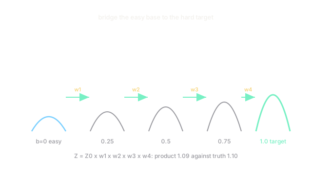
Annealed importance sampling (Neal, 2001) builds a bridge. Start from an easy distribution with known $Z_0$ , heat it through intermediates toward the target, move samples along with MCMC at each temperature, and multiply the stepwise ratios. The product estimates $Z$ unbiasedly. This page covers the constant and the annealing estimator; one-step importance sampling is the single-bridge special case, and posterior sampling itself is under Bayesian inference.

The one idea you need first

Importance sampling estimates $\mathbb{E}_p[f]$ from draws $q$ by weighting each draw with $p/q$ . When $q$ misses where $p$ concentrates, a few draws carry all the weight and the estimate collapses. Annealing fixes the mismatch gradually instead of in one jump.

Think of It Like This

Crossing a river on chained boats

You must cross a wide river but cannot jump it. Nobody can throw a rope across either. Instead a chain of boats anchors between the banks, each close enough to toss a rope to the next. You cross boat by boat, and the product of each small crossing's odds gives the odds of the whole trip.

The near bank is the easy base distribution, the far bank the target. Each boat is an intermediate temperature; adjacent boats overlap enough that one-step importance weights stay tame. A single leap (plain importance sampling) drowns when the banks are far apart.

How It Actually Works

Define intermediates $p_k(x) \propto p_0(x)^{1 - \beta_k} p_T(x)^{\beta_k}$ with $0 = \beta_0 < \beta_1 < \cdots < \beta_K = 1$ . Here $p_0$ is the easy base (known $Z_0$ ) and $p_T$ the target. One AIS run: draw $x_0$ from $p_0$ , then for each $k$ apply a transition $T_k$ leaving $p_k$ invariant, and accumulate

w = \prod_{k=1}^{K} \frac{\tilde{p}_k(x_{k-1})}{\tilde{p}_{k-1}(x_{k-1})}

with unnormalized densities $\tilde{p}$ . Average $w$ over runs times $Z_0$ estimates $Z_T$ unbiasedly. In log space the product becomes a sum, which is how it is implemented.

Worked example

Estimate $Z$ for $\tilde{p}_T(x) = \exp(-x^2/2) \times (1 + x^2/10)$ against base $p_0 = N(0,1)$ with $Z_0 = 1$ . True $Z = 1 + 1/10 = 1.1$ (since $\mathbb{E}_{N(0,1)}[x^2] = 1$ ). Use $K = 4$ temperatures $\beta = (0, 0.25, 0.5, 0.75, 1)$ . A typical run through $x = (0.5, 0.7, 0.4, 0.9)$ gives stepwise ratios about $(1.006, 1.012, 1.02, 1.05)$ , product $\approx 1.09$ . Average over $200$ runs lands near $1.10 \pm 0.03$ : the bridge recovers the constant one leap would have missed, since direct importance weights here have variance several times larger.

Schedule and diagnostics

Geometric or sigmoid $\beta$ schedules with $K$ in the hundreds to thousands are standard for real models. Diagnose with the effective sample size of the $w$ values: below a few percent of runs, add temperatures near where the stepwise variance spikes.

Code

1def ais_estimate(n_runs: int = 200) -> float:2    import random3    import math4    betas = [0.0, 0.25, 0.5, 0.75, 1.0]5    total = 0.06    for _ in range(n_runs):7        x = random.gauss(0, 1)  # draw from the base8        w = 1.09        for b_prev, b in zip(betas, betas[1:]):10            # Unnormalized intermediate densities at the current x.11            def tilde(bb: float) -> float:12                return math.exp(-0.5 * x * x) * (1 + bb * x * x / 10)13            w *= tilde(b) / tilde(b_prev)  # stepwise ratio14            x = random.gauss(x * 0.9, 0.4)  # short MCMC move toward p_b15        total += w16    return round(total / n_runs, 3)17
18
19print(ais_estimate())  # -> about 1.1 (typical draws give 1.07 to 1.13)

The mean over runs targets $Z = 1.1$ ; the comment records the typical band rather than a fixed digit, since sampling varies run to run.

Watch Out For

Averaging weights in raw space

AIS weights span orders of magnitude, so a naive mean overflows or underflows past a few dozen temperatures. Always accumulate $\log w$ and combine runs with log-sum-exp. If your estimate changes by factors of two when you reorder runs, you averaged in the wrong space.

Too few temperatures with a distant target

With $K$ tiny and a far target, one stepwise ratio carries everything and AIS degrades to plain importance sampling with all its variance. Symptoms: effective sample size under $1\%$ . Double $K$ (halving gaps) before adding runs; temperatures are cheaper than wasted samples.

The Quick Version

The normalizing constant $Z$ prices model comparison but resists plain Monte Carlo.
AIS bridges an easy base to the target through heated intermediates with MCMC moves.
The product of stepwise unnormalized ratios estimates $Z$ unbiasedly.
The worked bridge recovers $Z = 1.1$ within about $0.03$ over $200$ runs.
Implement in log space with log-sum-exp; raw-space averaging overflows.
Diagnose with effective sample size and add temperatures where stepwise variance spikes.