Online Learning and Regret

Why Does This Exist?

Batch learning assumes the dataset sits still while you study it. Spam filters, ad auctions and stock routers never get that luxury: each email, bid or tick arrives once, demands a decision now, and reveals the right answer only after. Retraining from scratch every round is hopeless, and assuming tomorrow looks like yesterday invites an adversary to punish exactly that.

Regret is the scoreboard built for this world. It compares your running total against the best single action chosen with full hindsight, and asks for procedures whose average gap shrinks to zero no matter how nasty the sequence. This page defines regret and proves the classic shrinking bound. The batch counterpart is maximum likelihood estimation; the optimizer this theory justifies is in stochastic gradient descent variants.

The one idea you need first

A loss $\ell_t(a)$ scores action $a$ on round $t$, revealed after you commit. Losses may be adversarial: chosen to hurt your rule, not drawn from any distribution. No statistical assumption saves you; only the algorithm's guarantee does.

Think of It Like This

How It Actually Works

On each round $t = 1, \ldots, T$ you pick an action (or a distribution over actions), then suffer loss $\ell_t$. Against $K$ fixed actions, your regret is:

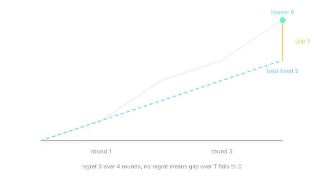
In plain words: your total minus the total of the best single action in hindsight. Note the benchmark never switches; beating a shifting target is much harder and needs Bandit-style extras. No regret means $R_T / T \to 0$: per-round you converge to the best fixed choice.

The workhorse is multiplicative weights. Keep a weight per action, play proportionally to weights, then multiply each weight by $(1 - \eta \ell_t(a))$ with step $\eta$. Good actions keep weight, bad ones decay exponentially. With $\eta = \sqrt{\log K / T}$ it guarantees $R_T \le \sqrt{T \log K}$: total regret grows like $\sqrt{T}$, so average regret falls like $1/\sqrt{T}$.

Worked example

Two news layouts A and B over $T = 4$ rounds. Miss-rate losses: A suffers $[0, 1, 0, 1]$ totalling $2$; B suffers $[1, 0, 1, 0]$ totalling $2$. A stubborn learner always picks A and totals $2$: regret $2 - 2 = 0$.

Now an adversary notices and flips the pattern against a copycat learner that always repeats last round's winner. Copycat picks B, A, B, A and suffers $[1, 1, 1, 1] = 4$. Best fixed is still $2$. Regret: $4 - 2 = 2$, average $0.5$ per round. Multiplicative weights with $\eta = 0.5$ instead splits weight toward both, totals about $2.7$ here, regret $0.7$: already far below $2$, and the $\sqrt{T \log 2}$ bound promises at most $\sqrt{4 \times 0.69} \approx 1.66$.

Code

Multiplicative weights on the copycat-trap sequence, showing regret well under the bound.

1import numpy as np2
3
4def hedge(losses: np.ndarray, eta: float) -> tuple[float, float]:5    w = np.ones(losses.shape[1])  # one weight per action6    total = 0.07    for row in losses:  # each round: play weights, then penalize8        p = w / w.sum()9        total += float(p @ row)10        w *= 1.0 - eta * row11    best = float(losses.sum(axis=0).min())12    return total, total - best13
14
15losses = np.array([[0.0, 1.0], [1.0, 0.0], [0.0, 1.0], [1.0, 0.0]])16print(hedge(losses, 0.5))  # -> (2.72, 0.72) approx, bound 1.66

Total about $2.7$ against best fixed $2$: regret $0.7$, inside the $1.66$ bound the theory promised.

Watch Out For

The Quick Version

• Online learning decides before seeing the loss; regret measures the gap to the best fixed action in hindsight.
• No regret means average regret tends to zero against any sequence, including adversarial ones.
• Multiplicative weights guarantees regret at most $\sqrt{T \log K}$ over $K$ actions and $T$ rounds.
• Copying the recent winner can suffer linear regret on alternating sequences.
• The benchmark is the best single action, not the best switching strategy.

What to Read Next

• Stochastic Gradient Descent Variants
• Convexity and Loss Landscapes
• Maximum Likelihood Estimation
• Information-Theoretic Generalization Bounds