Information-Theoretic Generalization Bounds

Generalisation costs information: the gap between test and train grows with how much the learned weights reveal about the training sample, measured by mutual information.

Weights holding 10 nats about the sample generalise within 0.10 while weights holding 100 nats allow gaps near 0.32

Why Does This Exist?

Stability and complexity bound the method or the class, but modern nets have huge classes yet leak little about training through noisy optimisation. What you want is a bound on the actual learned weights: if $W$ reveals almost nothing about sample $S$ beyond population structure, memorisation is impossible and the gap must be small. Mutual information $I(W; S)$ measures exactly that leakage in nats.

Xu-Raginsky made it rigorous: expected gap bounded by $\sqrt{2\sigma^2 I(W; S)/n}$ for $\sigma$ -sub-Gaussian loss. SGLD noise, compression and early stopping all shrink $I$ and tighten the bound. It also explains the information bottleneck preference for minimal sufficient representations: less information, smaller gap.

Prerequisite in one paragraph. You need mutual information $I(W;S)$ , the nats of dependence between weights and sample, and sub-Gaussian loss tails. Data processing says post-processing cannot create information. Background is in mutual information and data processing inequality.

Think of It Like This

A student who saw the exam versus one who learned the subject

Two students score $95$ on practice exams. One memorised answer keys: their brain holds $100$ nats about those exact sheets and collapses on new questions. The other learned methods: $10$ nats about the sheets, mostly shared structure, and repeats on finals.

Mutual information is the memorisation count. The bound charges the gap by $\sqrt{I/n}$ : the memoriser pays triple at the same $n$ . Noisy study habits, like SGLD, blur exact answers and force the second student's strategy.

Where the analogy stops: students choose strategies consciously while $I(W;S)$ is a property of the algorithm plus distribution. Estimating it for real nets needs bounds and proxies, not direct measurement.

How It Actually Works

Let $W$ be learned weights from sample $S$ of size $n$ and loss $\ell$ be $\sigma$ -sub-Gaussian in the relevant sense. Then $|E[L(W) - \hat{L}(W)]| \le \sqrt{2\sigma^2 I(W; S)/n}$ , where $L$ is test risk, $\hat{L}$ train risk and $I$ mutual information. Chaining across samples sharpens constants; conditional and disintegrated versions handle single draws rather than averages.

For SGLD with noise variance $\sigma_{\text{sgld}}^2$ over $T$ steps, $I$ grows like $(d/2)\log(1 + T\eta/d\sigma_{\text{sgld}}^2)$ -style quantities: more steps leak more, more noise leaks less. Compression bounds replace $I$ by description length: a $10$ -nat compressed model generalises almost as if $I = 10$ .

Worked example

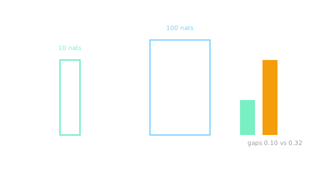
Take $n = 2000$ , $\sigma = 1$ . With $I = 10$ nats the bound gives $\sqrt{20/2000} = \sqrt{0.01} = 0.10$ . Train $0.15$ promises test below $0.25$ in expectation. With $I = 100$ nats it gives $\sqrt{200/2000} = \sqrt{0.10} \approx 0.316$ , diagram $0.32$ : same training, triple the allowed gap.

Halve to $n = 500$ with $I = 10$ : $\sqrt{20/500} = \sqrt{0.04} = 0.20$ . Information budgets interact directly with sample size, which is why compression helps most on small data.

Watch Out For

Estimating MI on the same data and quoting the bound

Plug-in MI estimates from training data are themselves overfit: they understate leakage because the estimator shares the memorisation. The bound with an underestimated $I = 2$ promises $0.045$ while true $I = 50$ allows $0.22$ .

Fix: bound $I$ analytically (SGLD, compression, VC-to-MI) or estimate on held-out randomization. Never plug a point estimate into its own bound.

Confusing representation MI with weights MI

$I(X; Z)$ for representations and $I(W; S)$ for weights bound different gaps through different theorems. Swapping them applies bottleneck intuition to weight leakage or vice versa, with mismatched $\sigma$ and $n$ scaling.

Fix: name both arguments of $I$ every time. Weights-sample bounds generalisation; input-representation bounds compression.

The Quick Version

Test-train gap scales as $\sqrt{I(W;S)/n}$ : leakage about the sample is the price.
Ten nats at 2000 samples hold the gap below 0.10; one hundred nats allow 0.32.
Noisy training, compression and early stopping shrink $I$ and tighten the bound.
Bound $I$ analytically; plug-in estimates on training understate it.
Weights-sample and input-representation informations answer different questions.