Optimal Transport in Generative Modeling

Optimal transport finds the cheapest way to morph one pile of probability into another, which gives generative models a stable distance and a straight training path between noise and data.

Two piles of probability mass pair up along the cheapest routes, and the total moving cost is the Wasserstein distance

Why Does This Exist?

Generative models must turn noise into data, but plain divergences misbehave. KL divergence explodes when the model puts zero mass where data lives, and it ignores geometry: shifting a generated image by one pixel can look identical yet score badly. Training needs a distance that stays finite when supports differ and grows with actual moving effort.

Optimal transport supplies it. It asks how much work it takes to rearrange one distribution into another, mass times distance, minimized over all pairings. That minimum is the Wasserstein distance, and it trains Wasserstein GANs, flow matching, and rectified flows. This page covers the transport problem and its 1D solution.

The one idea you need first

A coupling pairs every unit of mass in distribution $P$ with a destination in $Q$ . Many couplings exist; the cost of one is the average distance traveled under it. The optimal coupling is the cheapest pairing, and its cost is the distance between the distributions. Probability distributions carry the background.

Think of It Like This

Moving sand piles with wheelbarrows

Two sand piles sit in a yard: a round heap by the fence (noise) and a castle-shaped target (data). Any reshaping moves grains along paths, and each trip costs effort times distance. The cheapest full plan is optimal transport; its total bill is the Wasserstein distance.

Crossing paths waste effort, so the best plan never crosses: grains keep their order. Where the analogy stops: probability mass splits fractionally across destinations, which sand grains cannot, and entropy-regularized plans deliberately blur the assignment to compute faster.

How It Actually Works

For distributions $P$ and $Q$ with cost $c(x, y)$ , often $|x - y|^p$ , the $p$ -Wasserstein distance is:

W_p(P, Q) = \left( \min_{\pi} \mathbb{E}_{(x,y) \sim \pi}[c(x, y)] \right)^{1/p}

In plain words: $\pi$ ranges over couplings with marginals $P$ and $Q$ , the expectation totals the moving bill, and the minimum picks the cheapest plan. The choice $p = 1$ gives the earth mover distance; $p = 2$ gives smoother gradients and straight-line displacement paths used in flow matching.

In one dimension the answer is closed form: sort both samples and pair them in order. For empirical samples $x_{(1)} \le \dots \le x_{(n)}$ and $y_{(1)} \le \dots \le y_{(n)}$ , $W_1 = (1/n)\sum_i |x_{(i)} - y_{(i)}|$ . No linear program needed. In higher dimensions the Sinkhorn algorithm adds a small entropy bonus that makes the problem solvable by repeated row and column rescaling.

Worked example

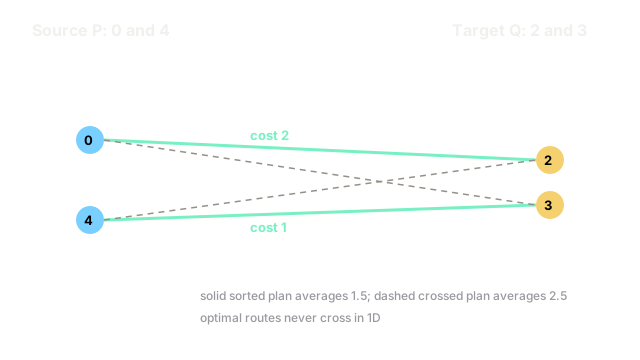
Move mass from $P = \{0, 4\}$ to $Q = \{2, 3\}$ , one unit each, cost is absolute distance.

Sorted pairing: $0 \to 2$ costs 2, $4 \to 3$ costs 1. Total $3$ , average $W_1 = 1.5$ . Crossed pairing: $0 \to 3$ costs 3, $4 \to 2$ costs 2, total $5$ , average $2.5$ . The sorted plan wins by $1.0$ , and no other pairing exists for two points. The optimal coupling keeps order, exactly as the sand picture predicts.

Code

1import numpy as np2
3
4def w1_sorted(x: np.ndarray, y: np.ndarray) -> float:5    xs = np.sort(x)  # optimal 1D plan pairs order statistics6    ys = np.sort(y)7    return float(np.mean(np.abs(xs - ys)))  # mean quantile gap8
9
10x = np.array([0.0, 4.0])11y = np.array([2.0, 3.0])12print(w1_sorted(x, y))  # -> 1.5

The output 1.5 matches the hand pairing. Try shuffling $y$ first and the sort inside still recovers the cheap plan, which is the entire 1D algorithm.

Watch Out For

Using Wasserstein where samples are too few

$W_1$ estimated from 50 samples in 100 dimensions mostly measures sampling noise, not distribution gap. The value stays large even for identical distributions because empirical clouds rarely overlap in high dimensions. Teams then chase a distance that cannot fall.

Fix it by using thousands of samples, reporting the sliced or entropic variant, or pairing the number with a fixed validation set. Never quote raw $W_1$ from a minibatch.

Forgetting the cost defines the distance

$W_2$ with squared Euclidean cost punishes long moves quadratically and yields straight paths, while $W_1$ with absolute cost tolerates them. Swapping costs mid-project changes rankings of models without changing any sample. The number is meaningless without the cost beside it.

Always state $p$ and the ground metric when you report the distance.

The Quick Version

Optimal transport is the cheapest pairing of two probability masses, and its cost is the Wasserstein distance.
In 1D the optimum sorts and pairs in order; the example $\{0,4\} \to \{2,3\}$ costs 1.5.
Sinkhorn adds entropy to make high-dimensional transport solvable by iterative rescaling.
Flow matching trains along the straight displacement paths that $W_2$ plans trace.
Always name the cost and use enough samples, since minibatch $W_1$ is mostly noise.