Math

Bayes' Theorem

The rule for flipping a conditional around — and the reason a highly accurate test for a rare thing still returns mostly false alarms.

A test that is ninety-nine percent accurate still yields mostly false alarms when the condition is rare: out of a million people the ninety-nine true positives are swamped by nearly ten thousand false ones

Why Does This Exist?

Your model flags 1,000 transactions as fraudulent and is right 99% of the time on the cases it has seen. How many of those 1,000 flags are actually fraud?

The answer is not 990, and if your on-call process assumes it is, your analysts will drown in false positives and stop reading the alerts. With fraud at roughly 1 in 1,000 transactions, most of those flags are wrong — not because the model is bad, but because there is so much more legitimate traffic to be wrong about. Bayes' theorem is the arithmetic that tells you this before you ship, and it is the reason precision and recall exist as separate metrics.

It also does something more structural. Every regularisation term you have ever used is a Bayesian prior in disguise. Weight decay is a Gaussian prior, L1 is a Laplace prior, and label smoothing is a prior on the targets. Once you have this page, maximum likelihood estimation and regularisation stop being two separate ideas and become one idea with an optional second term.

Think of It Like This

Hearing hoofbeats

You are in a European city and you hear hoofbeats behind you. Is it a horse or a zebra?

Zebras make an unmistakable sound, so the evidence fits a zebra as well as it fits a horse. But you do not conclude zebra, and the reason is not the evidence — it is that there were essentially no zebras in the city before you heard anything. Horses are rare here; zebras are very nearly absent.

Bayes' theorem is that reasoning made arithmetic. It multiplies two things: how well each explanation fits what you observed, and how plausible each explanation was to begin with. Strong evidence for something that was nearly impossible still comes out unlikely.

Now change one detail: you are standing outside a zoo. The evidence is identical and the answer flips, because only the prior moved. That is the part people skip, and it is the whole content of the theorem.

How It Actually Works

Start from the fact that "A and B" can be written two ways. From probability foundations, $P(A \cap B) = P(A \mid B)P(B)$ and equally $P(A \cap B) = P(B \mid A)P(A)$ . Set them equal and divide:

P(A \mid B) = \frac{P(B \mid A)\,P(A)}{P(B)}

In plain words: the chance of $A$ given $B$ is the chance of $B$ given $A$ , reweighted by how likely $A$ was beforehand and normalised by how likely $B$ was overall. That is the entire derivation — two lines, no new assumptions.

The four pieces have names you will meet constantly:

Posterior $P(A \mid B)$ — what you believe after seeing the evidence. The answer.
Likelihood $P(B \mid A)$ — how well the hypothesis explains the evidence.
Prior $P(A)$ — what you believed before. This is the term that gets forgotten.
Evidence $P(B)$ — how likely the observation was at all. Pure normalisation, and often the hard part.

The denominator is where the work is

$P(B)$ is usually not handed to you. You compute it by summing over every way $B$ could occur:

P(B) = P(B \mid A)P(A) + P(B \mid \neg A)P(\neg A)

In plain words: the evidence can arrive either because $A$ is true or because it is not, so add both routes. This is the law of total probability, and it is where the false positives enter the calculation — the second term is exactly "how often does this look positive when it is actually negative".

That term is also why Bayesian methods get computationally expensive. With continuous parameters the sum becomes an integral over every possible parameter value, and that integral usually has no closed form. Approximating it is what variational inference and MCMC are for.

Why the prior refuses to be ignored

Notice the posterior is proportional to likelihood times prior. If the prior is tiny, the posterior stays small no matter how well the evidence fits — a factor of 100 in likelihood cannot rescue a factor of 10,000 in prior.

This is the base-rate insight, and it generalises past medical tests. Rare-event detection is structurally precision-poor: anomaly detection, fraud, safety classifiers, rare disease screening, and any alert on a rare production failure. No accuracy improvement fixes it, because the problem is the ratio of populations, not the quality of the test. What fixes it is either raising the base rate before testing (screen a high-risk subgroup) or testing twice, where the first test's posterior becomes the second test's prior.

From posterior to loss function

Here is the connection that matters most for ML. Maximum likelihood picks the parameters $\theta$ maximising $P(D \mid \theta)$ . Bayes says you should instead maximise the posterior:

P(\theta \mid D) \propto P(D \mid \theta)\, P(\theta)

The evidence $P(D)$ does not depend on $\theta$ , so it drops out of the optimisation. Take logs and the product becomes a sum:

-\log P(\theta \mid D) = \underbrace{-\log P(D \mid \theta)}_{\text{your usual loss}} \; \underbrace{-\log P(\theta)}_{\text{the regularisation term}}

In plain words: your loss function plus a penalty for parameter values you considered implausible. Assume a zero-centred Gaussian prior on the weights and that second term works out to $\lambda \lVert \theta \rVert_2^2$ — L2 regularisation. Assume a Laplace prior and you get L1. This is MAP estimation, and it is why regularisation strength and prior confidence are the same dial.

Worked example

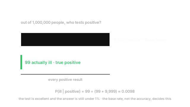
A disease affects 1 in 10,000 people. A test catches 99% of true cases and has a 1% false-positive rate. You test positive. What is the chance you are ill?

Work with a concrete population of 1,000,000 rather than symbols — it is faster and much harder to get wrong.

Ill: $1{,}000{,}000 / 10{,}000 = 100$ people. Of those, 99% test positive → 99 true positives.
Healthy: 999,900 people. Of those, 1% test positive → 9,999 false positives.

So 10,098 people test positive, and 99 of them are ill:

P(\text{ill} \mid \text{positive}) = \frac{99}{99 + 9{,}999} \approx 0.0098

Just under 1%. The test is genuinely good and the answer is still "probably not", because the healthy group is 10,000 times larger and its 1% error rate produces a hundred times more positives than the ill group produces in total.

Worth noting the update did work: you started at 1 in 10,000 (0.01%) and ended at about 1%, a hundredfold increase in belief. That is a large update. It is just a large update starting from nearly nothing.

Now test again, independently. The first posterior, 0.0098, becomes the new prior. Of 10,098 positives retested: the 99 ill give about 98 positives, the 9,999 healthy give about 100. So $P(\text{ill} \mid \text{two positives}) \approx 98/198 \approx 0.495$ — close to even. Two tests get you where intuition wrongly expected one to.

Show Me the Code

1def posterior(prior: float, sensitivity: float, false_positive: float) -> float:2    # Law of total probability in the denominator: the evidence can arrive3    # from a true case OR from a false alarm.4    true_pos = sensitivity * prior5    false_pos = false_positive * (1 - prior)6    return true_pos / (true_pos + false_pos)7
8
9p1 = posterior(prior=1 / 10_000, sensitivity=0.99, false_positive=0.01)10print(round(p1, 4))                                     # -> 0.0098  under 1%11
12# Sequential updating: yesterday's posterior is today's prior.13p2 = posterior(prior=p1, sensitivity=0.99, false_positive=0.01)14print(round(p2, 3))                                     # -> 0.495   near even15
16# Same excellent test, common condition: the base rate is doing the work.17print(round(posterior(0.10, 0.99, 0.01), 3))            # -> 0.917

The 0.0098 matches the hand calculation. The last line is the point of the whole page: identical test, prior moved from 1-in-10,000 to 1-in-10, and the answer moved from 1% to 92%.

Watch Out For

Quoting accuracy as if it were the posterior

"The model is 99% accurate" says nothing about how often its positive predictions are right. Those are different conditionals, and on rare events they differ by orders of magnitude.

The trap is sharper than it looks, because a 99%-accurate classifier on a 1-in-10,000 problem can be achieved by always predicting "negative" — that scores 99.99% accuracy and never detects anything. Accuracy on imbalanced data is close to meaningless, which is why precision, recall, and the precision–recall curve exist. Precision is the posterior: given a positive prediction, how often is it right.

In practice this decides whether a system is usable. A fraud model with 0.5% precision generates 200 alerts per genuine case, and no review team survives that. The number to negotiate with stakeholders is the expected count of false positives per day — an absolute number, computed from the base rate — not a percentage. Percentages hide base rates, and base rates are the whole problem.

Updating on evidence that is not independent

Sequential updating — posterior becomes the next prior — is valid only when each new observation is independent given the hypothesis. That condition fails more often than it holds.

Retest a patient with the same test and you often get the same result for the same underlying reason: an interfering substance, a sampling error, a systematic bias in the assay. The second test then adds far less information than the arithmetic claims, and chaining the updates produces a posterior far too confident. Two positives from independent tests took us to 49.5%; two positives from a test with a correlated failure mode might justify barely more than one.

The same failure shows up in ML pipelines. Ensemble members trained on the same data with the same architecture make correlated errors, so averaging their confidences overstates certainty. Retrieval-augmented systems that fetch several chunks from the same source document are not accumulating independent evidence. Anywhere you multiply likelihoods or chain updates, the question to ask is whether the failures are correlated — and if they are, the honest posterior is closer to the single-observation one than to the product.

The Quick Version

$P(A \mid B) = P(B \mid A)P(A) / P(B)$ — derived in two lines from the "and" rule, no new assumptions.
Posterior ∝ likelihood × prior. The prior is the term people drop, and it usually dominates.
The denominator is the law of total probability, summing over every route to the evidence. For continuous parameters it becomes an intractable integral.
A great test for a rare condition still yields mostly false positives. The base rate decides, not the accuracy.
Precision is the posterior. Accuracy is not, and on imbalanced data it is close to meaningless.
MAP estimation is maximum likelihood plus a prior; in log space the prior becomes a regularisation term.
L2 regularisation is a Gaussian prior. L1 is a Laplace prior.
Sequential updating requires conditionally independent observations. Correlated evidence makes the chained posterior overconfident.