The Rayleigh Quotient

One division that estimates an eigenvalue from any guess direction: put a vector in, get the energy per unit length out. Power iteration runs on it.

The quotient climbs from 4.0 toward 4.618 as the direction improves, because stationary points of the energy landscape sit exactly on eigenvectors

Why Does This Exist?

Eigenvalues are usually computed, not guessed. But iterative methods cannot afford a full decomposition: they hold one direction at a time and need a number from it. The Rayleigh quotient

R(x) = \frac{x^T A x}{x^T x}

turns any nonzero direction into an eigenvalue estimate. Point near an eigenvector and $R(x)$ lands near its eigenvalue; point at the eigenvector and it lands exactly. Power iteration, Rayleigh-quotient iteration and every variational eigenvalue argument run on this one division.

Its deeper content is stationary: the gradient of $R$ vanishes exactly at eigenvectors, so eigenvectors are the critical points of "energy per unit length" and eigenvalues are the critical values. The min-max theorem (Courant-Fischer) extends this to every eigenvalue, which is how eigenvalue bounds get proved.

The one idea you need first

The quadratic form $x^T A x$ measures energy along $x$ , and $x^T x = \lVert x \rVert^2$ measures squared length. Their ratio is energy per unit length, independent of how long $x$ is: $R(2x) = R(x)$ . Scale invariance is what makes the quotient a property of the direction, covered alongside sizes in norms.

Think of It Like This

Fuel efficiency of a route, not the fuel total

Two road trips burn different totals because one is longer. Divide by distance and you get litres per hundred kilometres: a property of the route and the car, comparable across trips of any length.

The Rayleigh quotient is litres-per-hundred for directions. $x^T A x$ is the trip total (it grows when $x$ grows); dividing by $x^T x$ removes length and leaves the direction's intrinsic number. Eigenvectors are the routes with extremal efficiency, and the quotient ranks every other direction between them.

How It Actually Works

Differentiate $R(x)$ and set the gradient to zero:

\nabla R = \frac{2Ax \cdot (x^T x) - 2x \cdot (x^T A x)}{(x^T x)^2} = 0 \iff Ax = R(x)\, x

Stationarity says $x$ is an eigenvector with eigenvalue $R(x)$ . So every critical point of the quotient is an eigenpair, and the global max over unit vectors is $\lambda_{\max}$ (attained at its eigenvector), the min $\lambda_{\min}$ . Better direction, better estimate, monotonically under power iteration.

Worked example

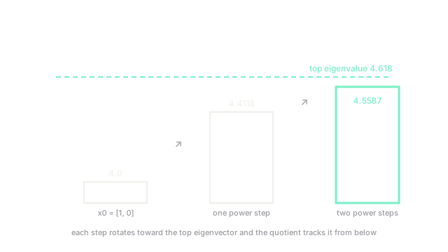
For $A = \begin{bmatrix} 4 & 1 \\ 1 & 3 \end{bmatrix}$ with $\lambda_{\max} \approx 4.618$ , feed three improving directions:

$x_0 = [1, 0]$ : $R = 4 / 1 = 4.0$
$x_1 = [0.9701, 0.2425]$ (one power step, normalised): $x_1^T A x_1 \approx 4.4118$ , so $R \approx 4.4118$
$x_2 = [0.9246, 0.3807]$ (two steps): $R \approx 4.5587$

The climb $4.0 \to 4.4118 \to 4.5587 \to 4.618$ shows the mechanism: each step rotates toward the top eigenvector and the quotient tracks it from below. Reversing the iteration (or negating $A$ ) climbs down to $\lambda_{\min}$ the same way.

Code

The point is the check: iterate the power method and watch the quotient converge from below.

1A = [[4.0, 1.0], [1.0, 3.0]]2
3
4def rayleigh(x: list[float]) -> float:5    ax = [A[0][0] * x[0] + A[0][1] * x[1], A[1][0] * x[0] + A[1][1] * x[1]]6    return (x[0] * ax[0] + x[1] * ax[1]) / (x[0] * x[0] + x[1] * x[1])7
8
9x = [1.0, 0.0]10vals = []11for _ in range(2):12    ax = [A[0][0] * x[0] + A[0][1] * x[1], A[1][0] * x[0] + A[1][1] * x[1]]13    n = (ax[0] ** 2 + ax[1] ** 2) ** 0.5  # renormalise each step14    x = [ax[0] / n, ax[1] / n]15    vals.append(round(rayleigh(x), 4))16print([round(rayleigh([1.0, 0.0]), 4)] + vals)  # -> [4.0, 4.4118, 4.5587]

Watch Out For

Using the quotient on a non-symmetric matrix

For non-symmetric $A$ , $R(x)$ can be complex-valued in effect and its stationary points need not be eigenvectors in any useful sense; the clean theory (real values, min-max, monotonicity) is symmetric-only. Check symmetry before variational arguments, or switch to singular values and the $A^T A$ quotient instead.

Maximising without the norm constraint

$x^T A x$ alone is unbounded above whenever any eigenvalue is positive: scale $x$ up and the "estimate" explodes. The denominator is load-bearing, not decoration. Unconstrained maximisation of a quadratic form diverges; always optimise the ratio or fix $\lVert x \rVert = 1$ explicitly.

The Quick Version

$R(x) = x^T A x / x^T x$ is energy per unit length: an eigenvalue estimate from any direction.
Stationary points sit exactly on eigenvectors, with the quotient equal to the eigenvalue.
Power steps climb $4.0 \to 4.4118 \to 4.5587 \to 4.618$ toward the top of the worked matrix.
The clean theory is symmetric-only; non-symmetric matrices need singular values instead.
Never maximise the numerator alone: without the denominator it diverges.