Reinforcement Learning Theory

RL theory studies how agents learn from rewards over time, giving the equations, convergence guarantees, and sample costs behind every practical algorithm.

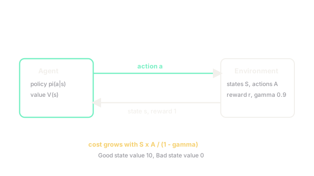
An agent loops through states, actions, and rewards while theory bounds how many trips around the loop learning needs

Why Does This Exist?

Reinforcement learning works in demos and wobbles in production: same algorithm, new task, wildly different data needs. Without theory you cannot tell whether a failure is a bug, a bad hyperparameter, or a task that fundamentally needs a million more episodes. Practitioners burned weeks on each possibility before the bounds existed.

Theory organizes the field around three questions. What is optimal (Bellman equations), will an algorithm reach it (convergence of dynamic programming and TD), and what does it cost (sample complexity and regret). This overview maps those three pillars and points to the dedicated pages for each mechanism.

The one idea you need first

A Markov decision process has states $s$ , actions $a$ , transition probabilities $P(s'|s,a)$ , rewards $r$ , and discount $\gamma$ in $[0,1)$ . The future depends only on the current state and action, never the full history. A policy $\pi(a|s)$ picks actions, and its value $V^\pi(s)$ is expected discounted return from $s$ . Markov chains carry the background.

Think of It Like This

Learning the fastest commute by trial

You move to a new city and must reach work fast. Each morning you pick a route (action), sit in traffic (transition), and clock your arrival (reward). After weeks you learn which turn pays off, discounting far-future shortcuts because traffic changes.

Theory is the city planner's version: the optimal route map (Bellman), proof your trial habit converges (TD theory), and the number of mornings you must suffer (sample complexity). Where the analogy stops: real commutes are nonstationary in ways MDP theory assumes away, so bounds describe the model, not the roadworks.

How It Actually Works

The optimal value $V^*$ satisfies the Bellman optimality equation:

V^*(s) = \max_a \left[ r(s,a) + \gamma \sum_{s'} P(s'|s,a) V^*(s') \right]

In plain words: the best you can do from $s$ is the best action's immediate reward plus the discounted best you can do after. The Bellman backup operator behind this equation contracts distances by $\gamma$ , so repeated backups converge to $V^*$ geometrically. That contraction is why planning works and is covered on its own page.

Learning splits by what is known. With a known model, dynamic programming applies backups directly. With samples only, temporal-difference methods apply noisy backups and average the noise away, which needs step sizes that sum to infinity while their squares sum finitely. Costs scale with states $S$ , actions $A$ , horizon $1/(1-\gamma)$ , and accuracy $1/\epsilon^2$ in the tabular case.

Worked example

Two states, Good and Bad. From Good, action Stay pays 1 and stays; action Risk pays 0 but jumps to Bad with probability 0.5. From Bad every action pays 0 and returns to Good with probability 0.5. Take $\gamma = 0.9$ .

Guess $V(G) = 10$ , $V(B) = 0$ . Stay from Good: $1 + 0.9 \times 10 = 10$ . Risk: $0 + 0.9(0.5 \times 10 + 0.5 \times 0) = 4.5$ . Stay wins, confirming $V(G) = 10$ since $1/(1-0.9) = 10$ . The Bellman equation certifies the cautious policy without simulating a single episode.

Watch Out For

Quoting tabular bounds for deep RL

Tabular sample bounds grow with $S \times A$ and assume every state revisits often. A pixel task has effectively infinite states, so the bound is vacuous and function approximation takes over with far weaker guarantees. Teams that promise tabular data budgets for Atari-scale tasks miss by orders of magnitude.

State which regime the bound assumes before using it to plan data collection.

Ignoring the discount in the horizon

Effective horizon is $1/(1-\gamma)$ : 10 steps at $\gamma = 0.9$ , 100 at $0.99$ . Doubling reported scores by raising $\gamma$ from 0.99 to 0.999 lengthens the horizon tenfold and the data need with it. Comparisons across papers with different $\gamma$ are not comparisons.

Fix $\gamma$ before comparing algorithms, and budget data with the horizon in mind.

The Quick Version

RL theory frames control as Markov decision processes with rewards, transitions, and discounting.
Bellman equations define optimal values, and their backup operator contracts by $\gamma$ .
Model-free methods apply noisy backups and need decaying step sizes to converge.
Tabular costs grow with states, actions, horizon, and inverse accuracy squared.
This page is the map; the contraction, policy gradient, TD, and exploration pages carry the proofs.