Stochastic Differential Equations

Equations that mix deterministic drift with Brownian noise. Their solutions are random paths whose means follow the drift and whose spreads follow the volatility.

Mean-reverting paths pull toward 5.0 while noise holds a steady band of width 0.25 after 2 time units

Why Does This Exist?

ODEs $dx/dt = \mu(x)$ describe exact motion, but markets wobble, sensors err and samplers inject noise deliberately. Adding a fixed noise trace to an ODE solution understates feedback: noise entering early propagates through later drift. The solution must be a random process defined jointly with its noise, not a deterministic curve plus frosting.

SDEs $dX = \mu\,dt + \sigma\,dW$ do that. They define Langevin samplers, Ornstein-Uhlenbeck models and the forward noising of diffusion generative models. Stochastic calculus and SDEs overviews the toolkit; diffusion processes studies their long-run behaviour and reverse-time SDEs run them backwards for generation.

Prerequisite in one paragraph. You need the Ito integral against $dW$ and Lipschitz drift for existence: $|\mu(x) - \mu(y)| \le L|x - y|$ keeps paths from exploding. Background is in Brownian motion and the Ito integral.

Think of It Like This

A thermostat in a draughty room

A thermostat pulls temperature toward $5$ degrees with strength proportional to the gap (drift), while draughts gust randomly (diffusion). The room never sits still: it wanders in a band around the setting, wider when draughts strengthen, narrower when the thermostat stiffens.

SDE solutions live in that band. Drift centres, noise spreads, and the stationary width balances the two. Crank the thermostat (mean reversion) and the band tightens; open windows (volatility) and it widens.

Where the analogy stops: rooms have bounded air while SDE paths are unbounded with Gaussian tails. Thermostats also switch discretely; SDE drift acts continuously.

How It Actually Works

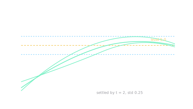
An SDE $dX_t = \mu(X_t)\,dt + \sigma(X_t)\,dW_t$ with initial $X_0$ has a unique strong solution when $\mu, \sigma$ are Lipschitz and grow at most linearly. The Ornstein-Uhlenbeck prototype $dX = \theta(m - X)\,dt + \sigma\,dW$ pulls toward level $m$ at speed $\theta$ . Its mean satisfies $dE[X]/dt = \theta(m - E[X])$ and its variance settles at $\sigma^2/2\theta$ .

Euler-Maruyama discretises with $X_{k+1} = X_k + \mu(X_k)\Delta + \sigma(X_k)\sqrt{\Delta}Z_k$ for standard normal $Z_k$ and step $\Delta$ . Halving $\Delta$ halves the weak error.

Worked example

Take $\theta = 2.0$ , $m = 5.0$ , $\sigma = 0.5$ starting $X_0 = 0$ . Mean path: $E[X_t] = 5(1 - e^{-2t})$ . At $t = 2$ , $e^{-4} \approx 0.0183$ , so mean $\approx 5 \times 0.9817 = 4.91$ . Stationary variance $\sigma^2/2\theta = 0.25/4 = 0.0625$ , standard deviation $0.25$ . After $2$ units paths sit in $5.0 \pm 0.5$ with chance about $0.95$ . The diagram band shows that width: drift did the centring, $\sigma$ set the $0.25$ scale, $\theta$ the $2$ -unit settling time.

Watch Out For

Simulating with too large a step on stiff drift

With $\theta = 20$ and $\Delta = 0.2$ , Euler-Maruyama multiplies by $1 - \theta\Delta = -3$ per step and explodes oscillatory, while the true process is stable. Stability needs $\theta\Delta$ well below $1$ .

Fix: keep $\Delta$ below $0.1/\theta$ for explicit Euler or switch implicit for stiff drifts. Check one stationary variance before long runs.

Reading pathwise convergence from weak convergence

Halving $\Delta$ halves weak error (means, moments) but strong pathwise error shrinks only as $\sqrt{\Delta}$ . Judging a sampler by single paths looks slow while its moments already converged.

Fix: match error type to use. Densities and means need weak; pathwise couplings need strong with finer steps.

The Quick Version

SDEs define random paths jointly with their driving noise, not ODE curves plus frosting.
Lipschitz drift plus linear growth guarantee a unique solution; Euler-Maruyama steps need small $\Delta$ .
Ornstein-Uhlenbeck with speed 2.0 and noise 0.5 centres at 5.0 with stationary standard deviation 0.25.
After 2 units the mean sits at 4.91 inside a 0.5 band with chance 0.95.
Stiff drifts need tiny or implicit steps, and weak versus strong errors scale differently.