Math

Taylor Series and Local Approximation

Replace a complicated function near one point with a simple polynomial that matches it there — the trick behind every optimisation step you have ever taken.

A straight line copies a curve's slope at one point and drifts away immediately; adding a curvature term keeps the approximation useful over a far wider range

Why Does This Exist?

Gradient descent takes a step in the direction of the negative gradient. Why should that work? The loss surface is not a straight line, and the gradient only describes one point on it.

Taylor's answer: near any point, a curved function behaves like a straight one. The gradient step is the minimiser of the first-order Taylor approximation, restricted to a small neighbourhood. That is the entire justification, and it also explains the failure mode — take too large a step and you have left the region where the approximation holds, which is exactly what a too-high learning rate does.

Keep one more term and you get Newton's method, which uses curvature and converges dramatically faster. Understanding why nobody uses it on a 7-billion-parameter model, and what Adam approximates instead, both start here. This is the missing rung between derivatives and curvature.

Think of It Like This

Describing a hill to someone by radio

You are standing on a hillside describing the terrain to someone who cannot see it.

The cheapest useful sentence is "it slopes down to the east at about one in five." They can now predict the ground a few metres away quite well. Further out they will be wrong, because you told them about a slope and the hill is curved.

Add a second sentence: "and it is getting steeper as you go." Now they can predict much further, because you have given them the rate at which the slope itself changes. Their mental picture bends the right way.

Keep going — "and the steepening eases off" — and the description gets more accurate over a wider range, at the cost of more to say.

That progression is a Taylor series. Each extra term buys accuracy further from where you are standing. And the crucial point is that the first sentence is enough if you only intend to take a small step, which is why one derivative is usually all training needs.

How It Actually Works

The Taylor series of $f$ around a point $a$ is:

f(x) = f(a) + f'(a)(x-a) + \frac{f''(a)}{2!}(x-a)^2 + \frac{f'''(a)}{3!}(x-a)^3 + \cdots

In plain words: the value at $a$ , plus the slope times how far you moved, plus a curvature correction, plus progressively finer corrections. Each term uses one more derivative at the single point $a$ — so the whole infinite series is built from local information.

Truncating gives approximations of increasing quality. Writing $h = x - a$ for the step:

Zeroth order: $f(a)$ . Error grows like $h$ .
First order: $f(a) + f'(a)h$ . This is the tangent line, and its error grows like $h^2$ .
Second order: adds $\tfrac{1}{2}f''(a)h^2$ . Error like $h^3$ .

The pattern matters more than the formulas: halving the step size cuts a first-order error by four and a second-order error by eight. Small steps make crude approximations excellent, which is the whole reason a learning rate exists.

The multivariable form is where ML lives

With a parameter vector $\theta$ and a step $d$ :

\mathcal{L}(\theta + d) \approx \mathcal{L}(\theta) + \nabla \mathcal{L}^{T} d + \tfrac{1}{2} d^{T} H d

Three terms, and each is a familiar object. $\mathcal{L}(\theta)$ is your current loss. $\nabla\mathcal{L}$ is the gradient. $H$ is the Hessian, holding the curvature.

Every optimiser is a choice about which terms to keep.

Keep only the first two and the approximation is linear, so it has no minimum — it decreases forever in the direction $-\nabla\mathcal{L}$ . You must therefore limit the step size, and that limit is the learning rate:

d = -\eta \nabla \mathcal{L}

Gradient descent is the minimiser of the first-order model inside a small trust region. The learning rate is the trust region.

Keep the curvature term and the quadratic model has a genuine minimum. Differentiating with respect to $d$ and setting to zero gives $Hd = -\nabla\mathcal{L}$ , so:

d = -H^{-1}\nabla \mathcal{L}

That is Newton's method. No learning rate is needed — the curvature sets the step length automatically, taking long steps in flat directions and short ones in steep directions. It converges quadratically near a minimum, meaning the number of correct digits roughly doubles each iteration.

Why nobody uses Newton's method on a large model

Three reasons, and they compound:

Memory. $H$ is $n \times n$ . At 7 billion parameters that is $4.9 \times 10^{19}$ entries.
Cost. Inverting it, or solving the linear system, is $O(n^3)$ .
Correctness. Newton's step is only a descent direction when $H$ is positive definite. At a saddle — which dominates high-dimensional landscapes — it can step confidently uphill.

So practical optimisers approximate the curvature cheaply. Adam and RMSProp keep a per-parameter second-moment estimate, which acts as a diagonal approximation to $H$ — one number per parameter instead of $n^2$ . L-BFGS keeps a low-rank approximation from recent gradients. Both are Taylor's second term, made affordable.

Worked example

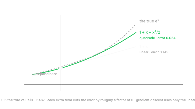
Expand $f(x) = e^{x}$ around $a = 0$ . Every derivative of $e^x$ is $e^x$ , and $e^0 = 1$ , so all coefficients are 1:

e^{x} \approx 1 + x + \frac{x^2}{2} + \frac{x^3}{6} + \cdots

Evaluate at $x = 0.5$ , where the true value is $e^{0.5} = 1.64872$ :

Order 0: $1$ — error $0.6487$
Order 1: $1 + 0.5 = 1.5$ — error $0.1487$
Order 2: $1.5 + 0.125 = 1.625$ — error $0.0237$
Order 3: $1.625 + 0.02083 = 1.64583$ — error $0.00289$

Each term cuts the error by roughly a factor of six. That is the diagram: the tangent line drifts off almost immediately while the quadratic tracks the curve much further.

Now watch the step size do its work. At $x = 0.1$ the true value is $1.10517$ , and the first-order estimate is $1.1$ — an error of $0.00517$ , about 29 times smaller than at $x = 0.5$ . The step shrank by 5 and the first-order error shrank by roughly $5^2 = 25$ , as the $h^2$ rule predicts.

That is the quantitative version of "small learning rates are safer": the crude linear model is genuinely accurate when the step is small, and genuinely wrong when it is not.

Show Me the Code

1import math2
3
4def taylor_exp(x: float, order: int) -> float:5    # Every derivative of e^x at 0 equals 1, so the coefficients are 1/k!.6    return sum(x**k / math.factorial(k) for k in range(order + 1))7
8
9true = math.exp(0.5)10print(round(true, 5))                                    # -> 1.6487211for order in range(4):12    est = taylor_exp(0.5, order)13    print(order, round(est, 5), round(abs(true - est), 5))14# -> 0 1.0 0.64872 | 1 1.5 0.14872 | 2 1.625 0.02372 | 3 1.64583 0.0028915
16# Halving the step should quarter the first-order error (it grows like h^2).17for h in (0.5, 0.25, 0.125):18    err = abs(math.exp(h) - taylor_exp(h, 1))19    print(h, round(err, 6))              # -> 0.148721, 0.034025, 0.008130

The errors match the hand calculation. The last block is the $h^2$ law: 0.1487 → 0.0340 → 0.0081, each roughly a quarter of the last, which is why step size controls approximation quality so directly.

Watch Out For

Assuming the local model holds over a large step

The Taylor approximation is only valid near the expansion point, and "near" depends on how curved the function is — a quantity you generally do not know.

This is the real content of a learning rate being too high. Your optimiser computed a descent direction from a linear model of the loss, then walked far enough that the model no longer described the terrain. The loss goes up, and repeated overshooting produces the oscillating or diverging loss curve everyone recognises. The gradient was correct; the extrapolation was not.

Adaptive methods are attempts to infer the safe step size. Line search evaluates the loss at candidate step lengths and backtracks until it actually decreases — reliable but expensive per step, since each trial is a forward pass. Trust-region methods maintain an explicit radius and shrink it when a step underperforms its prediction. Learning-rate warmup does something similar for a different reason: early in training the curvature is large and poorly estimated, so small steps are safer until the estimates settle.

The diagnostic worth internalising: if the loss rises from the very first step and lowering the learning rate makes it rise more slowly rather than falling, suspect a sign error instead. A too-large step diverges; a wrong sign climbs steadily.

Adding a curvature term without checking it is positive

Newton's step $d = -H^{-1}\nabla\mathcal{L}$ minimises the quadratic model — and only minimises it when $H$ is positive definite. At a saddle point, where the Hessian has both positive and negative eigenvalues, the quadratic model has no minimum at all, and the Newton step can point uphill with complete confidence.

This is not an edge case in deep learning. Saddles vastly outnumber local minima in high dimensions, because being a minimum requires every one of millions of eigenvalues to be positive. So a naive second-order method spends much of its time at points where its own model is invalid.

The standard repairs all amount to forcing positive definiteness. Damping solves $(H + \lambda I)d = -\nabla\mathcal{L}$ , shifting every eigenvalue up by $\lambda$ — the same $\lambda I$ trick as ridge regression, and it smoothly interpolates between Newton at $\lambda = 0$ and gradient descent at large $\lambda$ . Trust-region Newton limits the step so the model stays trustworthy. And saddle-free Newton uses the absolute values of the eigenvalues, so negative-curvature directions become descent directions instead of ascent ones.

Adam sidesteps the issue by using squared gradients rather than true second derivatives — always positive by construction, so it cannot produce an ascent direction this way. That is a real advantage of a crude approximation over a precise one.

The Quick Version

Taylor expands a function near a point into a polynomial built from its derivatives at that point.
Truncating at first order gives the tangent line, with error growing like $h^2$ ; second order gives error like $h^3$ .
Halving the step quarters the first-order error. That is why small steps make crude models accurate.
Multivariable form: $\mathcal{L}(\theta + d) \approx \mathcal{L} + \nabla\mathcal{L}^{T}d + \tfrac{1}{2}d^{T}Hd$ .
Gradient descent minimises the first-order model inside a trust region — and the learning rate is that trust region.
Keeping the curvature term gives Newton's method, $d = -H^{-1}\nabla\mathcal{L}$ , which needs no learning rate and converges quadratically.
Newton is impractical at scale: $n^2$ memory, $O(n^3)$ solve, and it is only a descent direction when $H$ is positive definite.
Adam and RMSProp are diagonal curvature approximations; L-BFGS is a low-rank one.
A too-large step means you left the region where your model was valid. Loss rising from step one is more likely a sign error.
Never trust a Newton step at a saddle. Damping, trust regions, or saddle-free variants fix it.