Math

Positive Definite Matrices

Matrices that curve upward in every direction — the property that makes a surface a bowl with one bottom, and the reason some optimisation problems are easy.

The signs of a matrix's eigenvalues decide the shape of the surface it defines: all positive gives a bowl with one bottom, mixed signs give a saddle with no bottom at all

Why Does This Exist?

This is the property that separates optimisation problems you can solve from ones you can only approximate.

When a loss function's Hessian is positive definite everywhere, the loss is convex: one minimum, reachable from any starting point, no dependence on initialisation or random seed. Linear regression, logistic regression, and SVMs are all in this category, which is why they train reproducibly. Neural networks are not, and every hidden layer with a nonlinearity is what destroys it.

It shows up in three more places you use directly:

Every covariance matrix is positive semi-definite. That is not a convention, it is forced by the definition, and it is why a computed covariance with a negative eigenvalue is always a bug.
Gaussian distributions require a positive definite covariance. Sampling from a multivariate normal needs a Cholesky factorisation, which only exists for positive definite matrices — so a badly conditioned covariance breaks sampling with a confusing error.
Ridge regularisation works by forcing it. Adding $\lambda I$ to $X^{T}X$ makes it positive definite by construction, which is why ridge always has a unique solution while ordinary least squares may not.

Think of It Like This

Three shapes of valley

You are dropped somewhere on a landscape in the dark, told to walk downhill, and asked where you will end up.

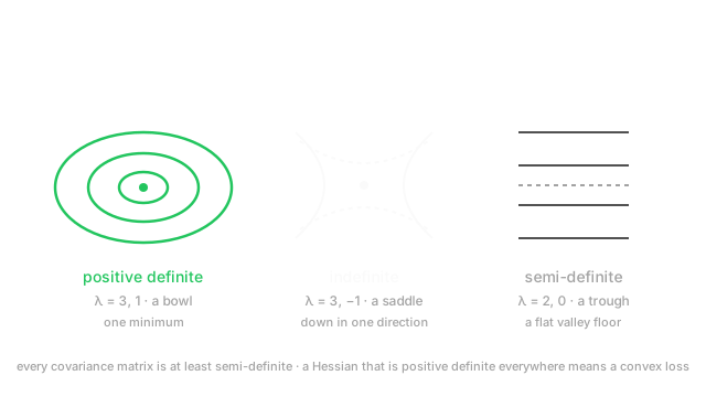
On a bowl, the answer is easy: there is exactly one bottom, and walking downhill from anywhere finds it. Every direction from the bottom goes up. That is positive definite.

On a saddle — think a mountain pass — the answer depends entirely on where you started. Walk downhill and you descend into one valley or the other, and there is no single bottom. Some directions from the middle go up, some go down. That is indefinite.

On a trough — a valley with a perfectly flat floor running along it — you reach the floor and then have nowhere to go. Every point along that floor is equally low, so "the" minimum is a whole line of them. That is semi-definite, with a zero eigenvalue marking the flat direction.

The eigenvalues are literally the curvature along each principal direction. All positive means every direction curves up: a bowl. One negative means one direction curves down: a saddle. One zero means one direction is flat: a trough.

How It Actually Works

The property is about a quadratic form — the scalar you get by sandwiching a vector around the matrix:

q(x) = x^{T} A x

In plain words: multiply the matrix by the vector, then dot the result back with the vector. The answer is one number, and the sign of that number for every possible $x$ is what defines the categories.

For a symmetric matrix $A$ :

Positive definite — $x^{T}Ax > 0$ for every nonzero $x$ . All eigenvalues positive.
Positive semi-definite (PSD) — $x^{T}Ax \ge 0$ for all $x$ . All eigenvalues $\ge 0$ , at least one zero.
Indefinite — the form takes both signs. Eigenvalues of mixed sign.
Negative definite — $x^{T}Ax < 0$ always. All eigenvalues negative.

Symmetry matters: for non-symmetric matrices only the symmetric part $(A + A^{T})/2$ affects the quadratic form, so the property is only ever discussed for symmetric matrices.

Four equivalent tests

These all say the same thing, and knowing which to reach for is the practical skill:

All eigenvalues positive. Conceptually the clearest, and $O(n^3)$ to check.
A Cholesky factorisation exists — $A = LL^{T}$ with $L$ lower-triangular and positive diagonal. This is the test to use in code: it is about twice as fast as an eigendecomposition and simply fails when the matrix is not positive definite.
All leading principal minors positive (Sylvester's criterion). Fine for $2 \times 2$ by hand, impractical otherwise.
$A = B^{T}B$ for some $B$ with full column rank. This is the constructive one, and it explains why so many matrices in ML are PSD.

That fourth form is worth dwelling on. $X^{T}X$ from least squares is PSD automatically, and positive definite exactly when $X$ has full column rank. A covariance matrix is $\frac{1}{n}X_c^{T}X_c$ for centred data, so it is PSD by construction. Gram matrices in kernel methods likewise. None of these are PSD by luck.

Why the property is so useful

It makes a quadratic have one minimum. Minimising $\frac{1}{2}x^{T}Ax - b^{T}x$ has gradient $Ax - b$ , so the stationary point solves $Ax = b$ . If $A$ is positive definite that point is the unique global minimum; if $A$ is indefinite it is a saddle and there is no minimum at all.

It classifies stationary points. At a point where the gradient is zero, the Hessian's definiteness tells you what you found: positive definite is a minimum, negative definite a maximum, indefinite a saddle. In high dimensions saddles vastly outnumber minima, because being a minimum requires every eigenvalue to be positive.

It guarantees invertibility. Positive definite means no zero eigenvalues, so the matrix is full rank and invertible. This is the whole mechanism of ridge regression: $X^{T}X$ may be singular, but $X^{T}X + \lambda I$ shifts every eigenvalue up by $\lambda$ , making them all strictly positive.

Worked example

Test two symmetric matrices.

A = \begin{bmatrix} 2 & 1 \\ 1 & 2 \end{bmatrix}, \qquad B = \begin{bmatrix} 1 & 2 \\ 2 & 1 \end{bmatrix}

For $A$ , the eigenvalues are 3 and 1 — both positive, so positive definite. Confirm with Sylvester: the first leading minor is $2 > 0$ , and the determinant is $4 - 1 = 3 > 0$ . Both positive ✓.

Check the quadratic form on the direction most likely to cause trouble, $x = [1, -1]$ . First $A x = [2 - 1,\; 1 - 2] = [1, -1]$ , then $x^{T}(Ax) = 1{\cdot}1 + (-1){\cdot}(-1) = 2 > 0$ ✓.

For $B$ , the characteristic polynomial is $(1-\lambda)^2 - 4 = 0$ , giving $\lambda = 3$ and $\lambda = -1$ . A negative eigenvalue, so indefinite — a saddle. Sylvester agrees: first minor $1 > 0$ , but the determinant is $1 - 4 = -3 < 0$ ✗.

Find the direction that proves it. Try $x = [1, -1]$ again: $Bx = [1 - 2,\; 2 - 1] = [-1, 1]$ , so $x^{T}(Bx) = 1{\cdot}(-1) + (-1){\cdot}1 = -2 < 0$ . Negative, so $B$ is definitively not PSD, and $[1,-1]$ is the downhill direction of the saddle.

Now the ridge repair. $C = \begin{bmatrix} 1 & 1 \\ 1 & 1 \end{bmatrix}$ has eigenvalues 2 and 0 — PSD but singular, a trough. Add $\lambda I$ with $\lambda = 0.5$ : eigenvalues become $2.5$ and $0.5$ , both positive, so $C + 0.5I$ is positive definite and invertible. Every eigenvalue shifted up by exactly $\lambda$ , which is the entire mechanism.

Show Me the Code

1import numpy as np2
3
4def is_positive_definite(A: np.ndarray) -> bool:5    # Cholesky is the fast test: it exists iff A is symmetric positive definite.6    try:7        np.linalg.cholesky(A)8        return True9    except np.linalg.LinAlgError:10        return False11
12
13A = np.array([[2.0, 1.0], [1.0, 2.0]])14B = np.array([[1.0, 2.0], [2.0, 1.0]])15C = np.array([[1.0, 1.0], [1.0, 1.0]])          # PSD but singular16
17print(np.linalg.eigvalsh(A), is_positive_definite(A))   # -> [1. 3.] True18print(np.linalg.eigvalsh(B), is_positive_definite(B))   # -> [-1. 3.] False19print(np.linalg.eigvalsh(C), is_positive_definite(C))   # -> [0. 2.] False20
21x = np.array([1.0, -1.0])22print(x @ A @ x, x @ B @ x)                     # -> 2.0 -2.0  the deciding direction23
24# Ridge: adding lambda*I shifts every eigenvalue up by lambda.25print(np.linalg.eigvalsh(C + 0.5 * np.eye(2)), is_positive_definite(C + 0.5 * np.eye(2)))26# -> [0.5 2.5] True

Every number matches the hand calculation. eigvalsh is used rather than eigvals because these matrices are symmetric — real values, sorted, faster.

Watch Out For

A covariance matrix with negative eigenvalues

Covariance is PSD by construction, so a negative eigenvalue is always a computational artifact — and it breaks everything downstream that assumes the property.

Three routes produce it. Catastrophic cancellation from the one-pass formula $E[XX^{T}] - E[X]E[X]^{T}$ , which is the same failure that makes one-pass variance return negative numbers. Pairwise deletion of missing values, where each entry is computed on a different subset, so the result is not a covariance of anything coherent. And plain accumulated rounding on a genuinely near-singular matrix, which lands eigenvalues at $-10^{-17}$ instead of 0.

The symptom is rarely a clear message. np.linalg.cholesky raises LinAlgError, sampling from a multivariate normal fails, or a Gaussian process fit crashes several layers away from the cause. People then blame the sampler.

Fixes, in order of preference. Compute covariance properly with np.cov rather than the one-pass identity. Use complete cases rather than pairwise deletion. And when a matrix is legitimately near-singular, add jitter: $\Sigma + \epsilon I$ with $\epsilon$ around $10^{-6}$ times the mean diagonal. That last one is standard practice in Gaussian process libraries and it is the same $\lambda I$ trick as ridge, applied for numerical rather than statistical reasons.

Checking definiteness by looking at the entries

There is no way to read positive definiteness off the entries, and two plausible-looking shortcuts are both wrong.

All-positive entries does not imply positive definite. $\begin{bmatrix} 1 & 2 \\ 2 & 1 \end{bmatrix}$ has every entry positive and an eigenvalue of $-1$ . It is the worked example above.

Some-negative entries does not imply not positive definite. $\begin{bmatrix} 2 & -1 \\ -1 & 2 \end{bmatrix}$ has negative off-diagonals and eigenvalues 1 and 3, so it is positive definite. Negative off-diagonals are completely normal in a covariance matrix — they mean the variables move oppositely.

The only reliable signal from the entries is a necessary condition: a positive definite matrix must have all diagonal entries positive, since $x^{T}Ax$ with $x$ a basis vector picks out $A_{ii}$ . So a non-positive diagonal entry rules it out immediately — but a positive diagonal proves nothing.

Test it properly. np.linalg.cholesky in a try block is the fast check; eigvalsh when you want to see how close to singular you are. And symmetrise first — A = (A + A.T) / 2 — because floating point leaves asymmetries that make the eigenvalue routines return complex results.

The Quick Version

The quadratic form is $x^{T}Ax$ , a single number. Its sign across all $x$ defines the category.
Positive definite: all eigenvalues positive, $x^{T}Ax > 0$ always. A bowl with one bottom.
PSD allows zeros (a flat trough); indefinite has mixed signs (a saddle).
Four equivalent tests: positive eigenvalues, Cholesky exists, positive leading minors, or $A = B^{T}B$ with full column rank.
Use Cholesky in code — twice as fast as eigendecomposition and fails cleanly.
$X^{T}X$ , covariance matrices and Gram matrices are PSD by construction, not coincidence.
Positive definite Hessian ⟹ that stationary point is a minimum. Mixed signs ⟹ saddle, and saddles dominate in high dimensions.
Positive definite ⟹ invertible. Ridge's $X^{T}X + \lambda I$ shifts every eigenvalue up by $\lambda$ , which is why ridge always has a unique solution.
A covariance with a negative eigenvalue is always a bug. Add jitter $\epsilon I$ when it is genuinely near-singular.
You cannot tell from the entries. All-positive entries can be indefinite; negative off-diagonals can be positive definite.