Universal Approximation Theorems

One wide hidden layer can mimic any well-behaved function if you give it enough units, which sets the floor every deeper result has to beat.

A sum of shifted bent units builds bumps that add up to any continuous curve, and adding units shrinks the leftover error

Why Does This Exist?

Before 1989, neural networks looked like a gamble: a flexible formula with no assurance it could even write down the function you wanted. The universal approximation theorems removed that first doubt. Cybenko, Hornik, and others proved that a feedforward net with one hidden layer and a squashing nonlinearity approximates any continuous function on a compact set, as closely as you like, given enough units.

That guarantee shapes everything after it. It tells you representation is rarely the binding constraint, which moves the hard questions to depth versus width (how many units does it take?) and to training (will gradient methods find the setting?). Without this floor, every failure would first raise the suspicion that the model class itself was too small.

The one idea you need first

A hidden unit computes $\sigma(w x + b)$ : a bent copy of the nonlinearity $\sigma$ (sigmoid, tanh, or ReLU), shifted by the bias $b$ and tilted by the weight $w$ . The output layer adds those bends with coefficients. So the whole network is a weighted sum of simple one-dimensional bumps and kinks.

Think of It Like This

Building any skyline from one brick shape

Imagine bricks that are all the same bent shape, but you may shift each brick left or right, stretch it, and stack them with different weights. With a handful you get stairs. With a few dozen you get arches and towers. With enough, you trace any skyline a visitor names, because each new brick fixes the worst remaining gap without wrecking the rest.

Hidden units are those bricks. The theorem says the set is complete: no skyline is out of reach. It does not say how many bricks a given skyline needs, or that a builder paid per brick would choose this material. That costing question belongs to depth-versus-width theory, and the builder's skill belongs to optimization.

How It Actually Works

Take one hidden layer with $n$ units and a continuous nonlinear $\sigma$ :

f_n(x) = \sum_{i=1}^{n} c_i \, \sigma(w_i x + b_i)

In plain words: coefficient $c_i$ sets how tall bump $i$ is, weight $w_i$ sets how steep, bias $b_i$ sets where it sits. With sigmoid $\sigma$ , each term is a soft step; differences of two steps make a bump; sums of bumps trace the target. With ReLU, each term is a kink; sums of kinks make piecewise-linear curves that hug any continuous target as kinks get dense.

The theorem's conditions matter. The target must be continuous and the domain compact (a closed bounded interval, not the whole line). The nonlinearity must be non-polynomial; a polynomial activation of fixed degree can only make polynomials, which cannot hug functions like $e^x$ uniformly. Width $n$ may need to be large: the theorem promises some $n$ works, with no usable bound on it.

Worked example

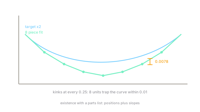
Approximate $f(x) = x^2$ on $[-1,1]$ with ReLU kinks to maximum error below $0.01$ . With $k$ equal pieces of width $2/k$ , linear interpolation of a parabola errs by at most $(2/k)^2 / 8 = 1/(2k^2)$ . Check: $k = 8$ gives $1/128 \approx 0.0078 < 0.01$ . So $8$ pieces, hence $7$ interior kinks and $8$ hidden units, suffice. Concretely, kinks at $x = -0.75, -0.5, \ldots, 0.75$ with matching slopes reproduce $x^2$ within eight thousandths everywhere. Existence becomes a shopping list: positions plus slopes.

Code

A piecewise-linear fit with kinks every $0.25$ reproduces the hand bound:

1def approx_square(x: float, kinks: list[float]) -> float:2    xs = [-1.0] + sorted(kinks) + [1.0]3    for a, b in zip(xs, xs[1:]):4        if a <= x <= b:5            return a * a + (x - a) * (b * b - a * a) / (b - a)  # chord between corners6    raise ValueError("x outside [-1, 1]")7
8
9grid = [i / 200 for i in range(-200, 201)]10kinks = [i / 4 for i in range(-3, 4)]11err = max(abs(approx_square(x, kinks) - x * x) for x in grid)12print(round(err, 4))  # -> 0.0078

Seven interior kinks give eight pieces and worst error $0.0078$ , matching the $1/(2k^2)$ bound computed by hand.

Watch Out For

Reading existence as efficiency

The theorem says some width works, even if that width is astronomically larger than your data. A target like a high-frequency sine wave on a wide interval can need exponentially many units shallowly while a deep stack builds it cheaply. If your one-layer net stalls, the fix is usually structure (depth, convolution, attention), not more units on the same layer.

Applying the theorem where its conditions fail

Discontinuous targets, unbounded domains, and polynomial activations each void the guarantee. A step function on $[0,1]$ is approximated poorly near the jump no matter the width (Gibbs-style overshoot with sigmoids, kink pile-up with ReLUs), and the error concentrates exactly where you likely care. Check continuity and compactness before blaming the optimizer.

The Quick Version

One hidden layer with a non-polynomial nonlinearity approximates any continuous function on a compact set.
The network is a weighted sum of shifted bent units: bumps with sigmoids, kinks with ReLUs.
Width $8$ traps $x^2$ within $0.008$ on $[-1, 1]$ , with kinks every $0.25$ .
The theorem promises existence with no usable bound on width and no training method.
Polynomial activations, discontinuous targets, and unbounded domains each break the guarantee.
Depth usually beats raw width on structured targets; that costing is a separate result.