Actor Critic using Kronecker-Factored Trust Region (ACKTR)

ACKTR scales natural policy gradients to deep networks by approximating the massive Fisher Information Matrix as Kronecker products of small activation and gradient covariance matrices.

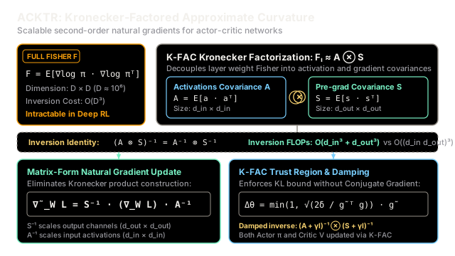
ACKTR decomposes the intractable network-wide Fisher information matrix into compact Kronecker factor matrices for activations and gradients, enabling fast second-order updates.

Why Does This Exist?

Standard first-order policy gradient methods, like Advantage Actor-Critic (A2C), update neural network parameters along the steepest Euclidean ascent direction. Because parameters govern policy distributions non-linearly, a uniform step in weight space can collapse the policy distribution from exploratory to near-deterministic in a single update.

Natural policy gradients solve this instability by measuring distance in probability distribution space via the Fisher Information Matrix (FIM), denoted $F$ . The natural gradient direction $\tilde{\nabla}_\theta J = F^{-1} \nabla_\theta J$ guarantees that step sizes represent invariant Kullback-Leibler (KL) divergences regardless of network parameterization.

However, for a network with $D \approx 10^6$ parameters, the FIM has dimension $D \times D$ ( $10^{12}$ elements). Directly storing and inverting $F$ demands $O(D^3) \approx 10^{18}$ floating-point operations per step, which is computationally impossible. While Trust Region Policy Optimization (TRPO) avoids constructing $F$ by approximating $F^{-1} g$ with iterative Conjugate Gradient steps, it requires repeated Hessian-vector passes and only optimizes the actor, leaving the critic to first-order Adam or RMSprop.

Actor Critic using Kronecker-Factored Trust Region (ACKTR) was introduced by Wu et al. (2017) to make exact second-order optimization practical for both the actor and the critic. By applying Kronecker-factored approximate curvature (K-FAC), ACKTR decomposes each layer's Fisher block into two compact covariance matrices: one over input activations and one over output pre-activation gradients. Inverting these tiny matrices reduces computational complexity from $O((d_{\text{in}} d_{\text{out}})^3)$ to $O(d_{\text{in}}^3 + d_{\text{out}}^3)$ , achieving two to three times the sample efficiency of TRPO and A2C without iterative conjugate gradient loops.

Think of It Like This

Measuring a Building by Floor Plan and Ceiling Height

Imagine you manage an auditorium renovation and need to adjust the acoustic damping of every seat. The auditorium has $d_{\text{in}} = 100$ rows and $d_{\text{out}} = 100$ columns, creating 10,000 seat adjustments ( $W \in \mathbb{R}^{100 \times 100}$ ).

A naive acoustician attempts to measure the pairwise acoustic interaction between every individual seat and every other seat across the room. That requires recording a $10{,}000 \times 10{,}000$ matrix with 100,000,000 cross-correlations, taking days to calculate and calibrate.

A master acoustic engineer notices the geometry: sound waves disperse independently along the row axis (input sound propagation) and along the column axis (vertical ceiling reflection). Rather than measuring 100 million pairwise interactions, she measures a $100 \times 100$ row-covariance matrix $A$ and a $100 \times 100$ column-covariance matrix $S$ .

To compute the necessary damping correction for any seat, she inverts the $100 \times 100$ row matrix and the $100 \times 100$ column matrix independently, then sandwiches the target adjustment between them: $S^{-1} G A^{-1}$ . She turns an intractable 100-million-parameter inversion problem into two split calibrations that execute in seconds.

Where the analogy stops: In a real auditorium, physical sound interactions across rows and columns can have higher-order cross-dependencies (e.g., sound bouncing diagonally off corners). K-FAC explicitly treats activations and output gradients as statistically independent when forming the expectation $\mathbb{E}[ (a a^\top) \otimes (s s^\top) ] \approx \mathbb{E}[a a^\top] \otimes \mathbb{E}[s s^\top]$ , accepting a slight structural approximation in exchange for massive computational tractability.

How It Actually Works

Natural Gradients and Kronecker-Factored Approximate Curvature

Consider a fully-connected layer in the actor or critic network mapping input activation $a \in \mathbb{R}^{d_{\text{in}}}$ to pre-activation outputs $s \in \mathbb{R}^{d_{\text{out}}}$ :

s = W a

Let $L$ denote the reinforcement learning surrogate objective, and define the pre-activation gradient $g_s = \nabla_s L$ . The gradient with respect to the weight matrix $W$ is an outer product:

\nabla_W L = g_s a^\top

Vectorizing the weight gradient gives:

\text{vec}(\nabla_W L) = a \otimes g_s

The Fisher Information Matrix block corresponding to layer weights $W$ is the expectation of the outer product of vectorized gradients:

F_l = \mathbb{E}\left[ \text{vec}(\nabla_W L) \text{vec}(\nabla_W L)^\top \right] = \mathbb{E}\left[ (a a^\top) \otimes (g_s g_s^\top) \right]

Computing the expectation of this Kronecker product directly couples activations and backward gradients. The K-FAC approximation assumes statistical independence between the activation covariance and the gradient covariance:

F_l \approx \mathbb{E}[a a^\top] \otimes \mathbb{E}[g_s g_s^\top] = A \otimes S

where:

$A = \mathbb{E}[a a^\top] \in \mathbb{R}^{d_{\text{in}} \times d_{\text{in}}}$ is the uncentered second moment of activations.
$S = \mathbb{E}[g_s g_s^\top] \in \mathbb{R}^{d_{\text{out}} \times d_{\text{out}}}$ is the uncentered second moment of pre-activation derivatives.

The crucial mathematical property that makes K-FAC scalable is that the inverse of a Kronecker product is the Kronecker product of the individual inverses:

F_l^{-1} \approx (A \otimes S)^{-1} = A^{-1} \otimes S^{-1}

To obtain the vectorized natural gradient $\text{vec}(\tilde{\nabla}_W L) = (A^{-1} \otimes S^{-1}) \text{vec}(\nabla_W L)$ , we leverage the matrix-vector identity $(B \otimes C) \text{vec}(X) = \text{vec}(C X B^\top)$ . Because $A$ is symmetric ( $A^{-\top} = A^{-1}$ ), the natural gradient in weight matrix form simplifies to:

\tilde{\nabla}_W L = S^{-1} (\nabla_W L) A^{-1}

Instead of inverting a $(d_{\text{in}} d_{\text{out}}) \times (d_{\text{in}} d_{\text{out}})$ matrix, ACKTR inverts one $d_{\text{in}} \times d_{\text{in}}$ matrix and one $d_{\text{out}} \times d_{\text{out}}$ matrix, followed by two fast matrix multiplications.

Trust Region Step and Covariance Running Averages

Running Statistics: Across parallel environment workers, empirical covariances are tracked with an exponential moving average (momentum parameter $\alpha \approx 0.95$ ):
$A_t = \alpha A_{t-1} + (1 - \alpha) \frac{1}{B} \sum_{i=1}^B a_i a_i^\top$ $S_t = \alpha S_{t-1} + (1 - \alpha) \frac{1}{B} \sum_{i=1}^B g_{s, i} g_{s, i}^\top$
Damped Inverses: To guarantee invertibility and numerical stability, Tikhonov damping $\gamma > 0$ is added:
$(A_t + \gamma I)^{-1}, \quad (S_t + \gamma I)^{-1}$
Trust Region Constraint: Let $\tilde{g}$ be the concatenation of all natural gradients across layers, and $g$ be the concatenated standard gradients. The KL divergence constraint per update is enforced by scaling the natural gradient step:
$\beta = \min\left(1, \sqrt{\frac{2\delta}{\tilde{g}^\top g}}\right)$ $\Delta \theta = \beta \tilde{g}$
where $\delta$ is the maximum allowed average KL divergence (typically $\delta \approx 0.01$ ).

Worked numerical example

Let us trace a concrete $2 \times 2$ layer ( $d_{\text{in}} = 2, d_{\text{out}} = 2$ ) step-by-step.

Suppose the accumulated activation covariance $A$ and pre-activation gradient covariance $S$ (including damping) are diagonal matrices:

A = \begin{bmatrix} 2.0 & 0.0 \\ 0.0 & 1.0 \end{bmatrix}, \quad S = \begin{bmatrix} 4.0 & 0.0 \\ 0.0 & 2.0 \end{bmatrix}

The first-order gradient matrix $\nabla_W L = G$ is:

G = \begin{bmatrix} 1.0 & 1.0 \\ 1.0 & 1.0 \end{bmatrix}

Invert Covariances:
$A^{-1} = \begin{bmatrix} 0.5 & 0.0 \\ 0.0 & 1.0 \end{bmatrix}, \quad S^{-1} = \begin{bmatrix} 0.25 & 0.0 \\ 0.0 & 0.5 \end{bmatrix}$
Compute Matrix-Form Natural Gradient:
$S^{-1} G = \begin{bmatrix} 0.25 & 0.0 \\ 0.0 & 0.5 \end{bmatrix} \begin{bmatrix} 1.0 & 1.0 \\ 1.0 & 1.0 \end{bmatrix} = \begin{bmatrix} 0.25 & 0.25 \\ 0.50 & 0.50 \end{bmatrix}$ $\tilde{G} = (S^{-1} G) A^{-1} = \begin{bmatrix} 0.25 & 0.25 \\ 0.50 & 0.50 \end{bmatrix} \begin{bmatrix} 0.5 & 0.0 \\ 0.0 & 1.0 \end{bmatrix} = \begin{bmatrix} 0.125 & 0.25 \\ 0.250 & 0.50 \end{bmatrix}$
Verify Equivalence with Full Kronecker Inverse: The full $4 \times 4$ Kronecker product $F = A \otimes S$ is:
$A \otimes S = \begin{bmatrix} 2.0 \cdot S & 0 \\ 0 & 1.0 \cdot S \end{bmatrix} = \text{diag}(8.0, 4.0, 4.0, 2.0)$
Its inverse is:
$(A \otimes S)^{-1} = \text{diag}(0.125, 0.25, 0.25, 0.50)$
The column-major vectorized gradient is $\text{vec}(G) = [1.0, 1.0, 1.0, 1.0]^\top$ . Applying the inverse:
$\text{vec}(\tilde{G}) = (A \otimes S)^{-1} \text{vec}(G) = [0.125, 0.25, 0.25, 0.50]^\top$
Reshaping back to a $2 \times 2$ matrix yields exactly $\begin{bmatrix} 0.125 & 0.25 \\ 0.25 & 0.50 \end{bmatrix}$ .
Apply Trust-Region Scaling: Let the KL constraint limit be $\delta = 0.01$ . The inner product between the natural gradient and the original gradient is:
$\tilde{g}^\top g = (0.125)(1.0) + (0.25)(1.0) + (0.25)(1.0) + (0.50)(1.0) = 1.125$
The scaling coefficient $\beta$ is:
$\beta = \min\left(1, \sqrt{\frac{2 \cdot 0.01}{1.125}}\right) = \min\left(1, \sqrt{0.017778}\right) \approx \min(1, 0.13333) = 0.13333$
The resulting parameter step $\Delta W = \beta \tilde{G}$ safely limits policy divergence.

Code

1import numpy as np2
3
4class KFACLinearOptimizer:5    """Computes Kronecker-factored natural gradients and trust-region updates6
7    for a linear feedforward layer W in R^{d_out x d_in}.8    """9
10    def __init__(11        self,12        d_in: int,13        d_out: int,14        damping: float = 1e-3,15        kl_clip: float = 0.01,16        alpha: float = 0.95,17    ) -> None:18        self.d_in = d_in19        self.d_out = d_out20        self.damping = damping21        self.kl_clip = kl_clip22        self.alpha = alpha23
24        # Covariance matrices initialized to identity25        self.cov_a = np.eye(d_in, dtype=np.float64)26        self.cov_s = np.eye(d_out, dtype=np.float64)27
28    def update_covariances(29        self,30        activations: np.ndarray,31        pre_grads: np.ndarray,32    ) -> None:33        """Updates running exponential moving averages of activation and gradient covariances.34
35        activations: shape (batch_size, d_in)36        pre_grads: shape (batch_size, d_out)37        """38        batch_size = activations.shape[0]39
40        # Empirical batch covariances: E[a a^T] and E[s s^T]41        batch_cov_a = (activations.T @ activations) / batch_size42        batch_cov_s = (pre_grads.T @ pre_grads) / batch_size43
44        self.cov_a = self.alpha * self.cov_a + (1.0 - self.alpha) * batch_cov_a45        self.cov_s = self.alpha * self.cov_s + (1.0 - self.alpha) * batch_cov_s46
47    def compute_natural_gradient(48        self,49        grad_w: np.ndarray,50    ) -> tuple[np.ndarray, np.ndarray]:51        """Computes natural gradient using fast matrix sandwich product S^{-1} G A^{-1}52
53        and compares it against the full Kronecker product inverse.54        """55        # Add Tikhonov damping56        a_damped = self.cov_a + self.damping * np.eye(self.d_in)57        s_damped = self.cov_s + self.damping * np.eye(self.d_out)58
59        # Invert d_in x d_in and d_out x d_out matrices60        inv_a = np.linalg.inv(a_damped)61        inv_s = np.linalg.inv(s_damped)62
63        # Fast matrix form: G_tilde = S^{-1} @ grad_w @ A^{-1}64        nat_grad_matrix = inv_s @ grad_w @ inv_a65
66        # Full Kronecker inverse verification67        kron_fim = np.kron(a_damped, s_damped)68        inv_kron_fim = np.linalg.inv(kron_fim)69        vec_grad = grad_w.flatten(order="F")70        vec_nat_grad = inv_kron_fim @ vec_grad71        nat_grad_kron = vec_nat_grad.reshape((self.d_out, self.d_in), order="F")72
73        return nat_grad_matrix, nat_grad_kron74
75    def step(self, grad_w: np.ndarray) -> tuple[np.ndarray, float]:76        """Calculates trust-region scaled natural gradient step."""77        nat_grad, _ = self.compute_natural_gradient(grad_w)78
79        # Inner product g^T * g_tilde across weights80        g_dot_gtilde = float(np.sum(grad_w * nat_grad))81
82        # Trust region factor beta = min(1, sqrt(2 * delta / (g^T g_tilde)))83        if g_dot_gtilde > 1e-12:84            scale = min(1.0, np.sqrt(2.0 * self.kl_clip / g_dot_gtilde))85        else:86            scale = 1.087
88        step_direction = scale * nat_grad89        return step_direction, scale90
91
92if __name__ == "__main__":93    np.set_printoptions(precision=4, suppress=True)94
95    # Initialize 2x2 layer optimizer96    opt = KFACLinearOptimizer(d_in=2, d_out=2, damping=0.0, kl_clip=0.01)97
98    # Manually assign covariance matrices matching the worked numerical example99    opt.cov_a = np.diag([2.0, 1.0])100    opt.cov_s = np.diag([4.0, 2.0])101
102    grad_w = np.ones((2, 2), dtype=np.float64)103
104    nat_grad_mat, nat_grad_kron = opt.compute_natural_gradient(grad_w)105    step_delta, scale_factor = opt.step(grad_w)106
107    print("Matrix Natural Gradient:")108    print(nat_grad_mat)109    # -> Matrix Natural Gradient:110    # -> [[0.125 0.25 ]111    # ->  [0.25  0.5  ]]112
113    print("\nVectorized Kronecker Gradient:")114    print(nat_grad_kron)115    # -> Vectorized Kronecker Gradient:116    # -> [[0.125 0.25 ]117    # ->  [0.25  0.5  ]]118
119    print(f"\nTrust Region Scaling Factor: {scale_factor:.6f}")120    # -> Trust Region Scaling Factor: 0.133333121
122    print("\nStep Direction:")123    print(step_delta)124    # -> Step Direction:125    # -> [[0.0167 0.0333]126    # ->  [0.0333 0.0667]]127
128    # Ensure matrix form matches Kronecker form129    assert np.allclose(nat_grad_mat, nat_grad_kron)130    print("\nVerification Passed: Matrix form matches exact Kronecker inverse.")131    # -> Verification Passed: Matrix form matches exact Kronecker inverse.

Watch Out For

Inversion Frequency Overhead and Damping Mismatch

Inverting $A$ and $S$ at every micro-step degrades computational throughput. In practice, ACKTR decouples the covariance update from matrix inversion: covariance running averages are accumulated on every mini-batch, but the costly matrix inversions $(A + \gamma I)^{-1}$ and $(S + \gamma I)^{-1}$ are recomputed only once every $T_{\text{inv}} \approx 20$ to 100 steps.

Furthermore, if the Tikhonov damping parameter $\gamma$ is chosen too small, empirical covariances can become near-singular, generating exploding gradient steps. Conversely, if $\gamma$ is excessively large, $(A + \gamma I)^{-1} \approx \gamma^{-1} I$ , collapsing the natural gradient back into standard vanilla gradient descent and sacrificing all second-order curvature benefits. Keep $\gamma$ calibrated to the variance of the policy distribution.

The Quick Version

Kronecker Factorization: ACKTR replaces the intractable $D \times D$ Fisher Information Matrix with layer-wise Kronecker products of input activations and output gradient covariances ( $F_l \approx A \otimes S$ ).
Inversion Scalability: Leveraging $(A \otimes S)^{-1} = A^{-1} \otimes S^{-1}$ reduces inversion complexity from $O((d_{\text{in}} d_{\text{out}})^3)$ to $O(d_{\text{in}}^3 + d_{\text{out}}^3)$ , allowing natural gradients to run on modern GPUs.
Actor and Critic Optimization: Unlike TRPO, which applies second-order updates only to the actor, ACKTR applies K-FAC natural gradient updates to both policy and value networks.
No Conjugate Gradients: Eliminates the iterative Hessian-vector multiplication loops required by TRPO, delivering higher sample efficiency with consistent wall-clock throughput.