Advantage Actor-Critic (A2C)

A2C reduces policy gradient variance by subtracting a learned baseline value from returns, evaluating whether actions performed better or worse than expected.

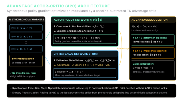
Why Does This Exist?

Pure policy gradient algorithms like REINFORCE optimize policies directly by sampling full trajectories and computing returns $G_t = \sum_{k=0}^\infty \gamma^k R_{t+k+1}$ . While the resulting policy gradient is theoretically unbiased, it suffers from catastrophic variance:

An identical action executed in an identical state can yield vastly different Monte Carlo returns depending on stochastic downstream transitions hundreds of steps into the future.
If all returns in an environment are strictly positive (e.g., $G_t \in [100, 150]$ ), REINFORCE increases the selection probability of every visited action, relying solely on relative gradient magnitudes to separate good choices from mediocre ones.

To reduce this variance, the policy gradient theorem permits subtracting any state-dependent baseline $b(s)$ that does not depend on action $a$ . Because $\sum_a \nabla_\theta \pi_\theta(a|s) = \nabla_\theta \sum_a \pi_\theta(a|s) = \nabla_\theta (1) = 0$ , baseline subtraction leaves the expected gradient strictly unbiased:

$\mathbb{E}_{a \sim \pi} \left[ \nabla_\theta \log \pi_\theta(a \mid s) b(s) \right] = 0$

The mathematically optimal baseline for minimizing variance is the state-value function $V(s)$ . Subtracting $V(s)$ from the action-value $Q(s, a)$ defines the Advantage Function:

$A(s, a) = Q(s, a) - V(s)$

The advantage measures whether taking action $a$ was better ( $A > 0$ ) or worse ( $A < 0$ ) than the average action expected under the current policy.

While early actor-critic algorithms like Asynchronous Advantage Actor-Critic (A3C, Mnih et al., 2016) used multiple independent CPU threads asynchronously writing updates to a shared central model without locks (Hogwild!), this approach suffered from race conditions, CPU bottlenecks, and GPU under-utilization. In 2017, researchers at OpenAI demonstrated that Advantage Actor-Critic (A2C)—the synchronous counterpart that steps $N$ parallel environments in lockstep—delivers identical or superior sample efficiency, achieves higher GPU utilization, and removes asynchronous threading artifacts.

Think of It Like This

The Director and the Script Editor

Imagine a film production set creating an improvised drama:

The Actor (The Director $\pi_\theta$ ): The director commands the actors on set, experimenting with scene improvisation, dialogue timing, and camera angles (actions).
The Critic (The Script Editor $V_\phi$ ): The script editor sits behind the monitor with an objective overview of the entire narrative arc. The editor does not choose the camera angles, but they maintain a baseline expectation of how dramatic and valuable the scene should be ( $V(s)$ ).

When the director calls "Cut!", the editor evaluates the take against the baseline:

Positive Advantage ( $\delta > 0$ ): The take exceeded expectations! The editor gives enthusiastic feedback: "That was brilliant—do more takes with that pacing!" The director reinforces that choice.
Negative Advantage ( $\delta < 0$ ): The take fell flat. Even if the scene was not an outright disaster, it fell short of the script's baseline expectation. The editor warns: "That dragged the pacing down—cut that line." The director dials back that choice.

Without the script editor (pure REINFORCE), the director would only know whether the entire finished movie won an award six months later, struggling to deduce which specific takes actually helped or hurt.

Where the analogy stops: Film directors rely on subjective artistic taste. In A2C, the critic minimizes the objective Bellman squared error towards discounted empirical rewards, mathematically proving that the advantage expectation is an unbiased variance-reduced policy gradient.

How It Actually Works

Advantage Formulation, Dual Objectives, and Synchronous Batches

The policy gradient theorem with a state-value baseline states:

$\nabla_\theta J(\theta) = \mathbb{E}_{\pi_\theta} \left[ \nabla_\theta \log \pi_\theta(A_t \mid S_t) A(S_t, A_t) \right]$

In practice, $Q(S_t, A_t)$ is unknown. Rather than maintaining a separate neural network for $Q$ , A2C uses the 1-step temporal difference (TD) error from the state-value critic $V_\phi(s)$ as an unbiased sample estimate of the advantage:

$\delta_t = R_{t+1} + \gamma V_\phi(S_{t+1}) - V_\phi(S_t)$

Taking the expectation conditioned on $(S_t, A_t)$ :

$\mathbb{E} \left[ \delta_t \mid S_t, A_t \right] = \mathbb{E} \left[ R_{t+1} + \gamma V_\phi(S_{t+1}) \mid S_t, A_t \right] - V_\phi(S_t) = Q(S_t, A_t) - V_\phi(S_t) = A(S_t, A_t)$

Thus, the 1-step TD error $\delta_t$ serves as a direct proxy for the advantage.

The Dual Optimization Objective

A2C trains two neural network heads (often sharing early feature extraction layers):

The Actor Objective (Policy Gradient + Entropy): The actor maximizes policy performance while maintaining exploration via an entropy regularization bonus: $\mathcal{L}_{\text{actor}}(\theta) = -\mathbb{E} \left[ \log \pi_\theta(A_t \mid S_t) \delta_t + \beta H(\pi_\theta(\cdot \mid S_t)) \right]$ where $H(\pi) = -\sum_a \pi(a \mid S_t) \log \pi(a \mid S_t)$ is the Shannon entropy, and $\beta > 0$ controls exploration pressure. Adding $-\beta H$ penalizes deterministic policies early in training, preventing the actor from prematurely collapsing into suboptimal actions.
The Critic Objective (Value Function Regression): The critic minimizes the mean squared Bellman error: $\mathcal{L}_{\text{critic}}(\phi) = \frac{1}{2} \mathbb{E} \left[ \left( R_{t+1} + \gamma V_\phi(S_{t+1}) - V_\phi(S_t) \right)^2 \right] = \frac{1}{2} \mathbb{E} \left[ \delta_t^2 \right]$
Combined Joint Loss: When training a shared neural network backbone with feature parameters $\psi$ , actor head $\theta$ , and critic head $\phi$ : $\mathcal{L}_{\text{total}}(\psi, \theta, \phi) = \mathcal{L}_{\text{actor}}(\theta) + c_1 \mathcal{L}_{\text{critic}}(\phi) - \beta H(\pi_\theta)$ where $c_1 \approx 0.5$ balances the critic loss magnitude against policy updates.

Synchronous Execution Architecture

Instead of running asynchronous worker threads that perform uncoordinated parameter updates on CPU (A3C), A2C steps $N$ parallel vectorized environments in lockstep:

All $N$ workers observe current states $[S_t^{(1)}, \dots, S_t^{(N)}]$ .
The GPU executes a single batched forward pass through actor $\pi_\theta$ and critic $V_\phi$ .
All $N$ workers execute their chosen actions simultaneously, returning next states and rewards.
Transitions are aggregated into a uniform mini-batch tensor of size $(N \times T)$ for efficient GPU backpropagation.

Worked numerical example

Consider a single transition step in an environment with a 2-dimensional continuous state representation and 2 discrete actions: $\mathcal{A} = \{a_0, a_1\}$ .

Current State Features: $\mathbf{x}(S_t) = [1.0, 0.5]^\top$ .
Next State Features: $\mathbf{x}(S_{t+1}) = [0.8, 1.2]^\top$ .
Reward: $R_{t+1} = 2.0$ , discount factor $\gamma = 0.9$ .
Critic: Linear parameter vector $\mathbf{w}_c = [0.5, 1.0]^\top$ .
Actor: Linear logits vector $\mathbf{z} = [0.6, 0.2]^\top$ .
Entropy Coefficient: $\beta = 0.01$ .

Step 1: Critic Evaluation and Advantage Computation

Current State Value: $V(S_t) = \mathbf{w}_c^\top \mathbf{x}(S_t) = 0.5(1.0) + 1.0(0.5) = 0.5 + 0.5 = 1.0000$
Next State Value: $V(S_{t+1}) = \mathbf{w}_c^\top \mathbf{x}(S_{t+1}) = 0.5(0.8) + 1.0(1.2) = 0.4 + 1.2 = 1.6000$
Temporal Difference Error (Advantage $\delta_t$ ): $\delta_t = R_{t+1} + \gamma V(S_{t+1}) - V(S_t) = 2.0 + 0.9(1.6000) - 1.0000 = 2.0 + 1.4400 - 1.0000 = 2.4400$ Interpretation: The observed transition produced an advantage of $+2.44$ , significantly outperforming the critic's baseline expectation.

Step 2: Actor Policy and Entropy Evaluation

Softmax Action Probabilities from logits $[0.6, 0.2]$ : $e^{0.6} \approx 1.8221, \quad e^{0.2} \approx 1.2214, \quad \sum = 3.0435$ $\pi(a_0 \mid S_t) = \frac{1.8221}{3.0435} \approx 0.5987, \quad \pi(a_1 \mid S_t) = \frac{1.2214}{3.0435} \approx 0.4013$
Suppose the agent executed action $A_t = a_0$ : $\log \pi(a_0 \mid S_t) = \log(0.5987) \approx -0.5130$
Policy Entropy $H(\pi)$ : $H(\pi) = - \left[ 0.5987 \log(0.5987) + 0.4013 \log(0.4013) \right]$ $H(\pi) = - \left[ 0.5987(-0.5130) + 0.4013(-0.9130) \right] = - \left[ -0.3071 - 0.3664 \right] = 0.6735$

Step 3: Compute Loss Quantities

Actor Loss: $\mathcal{L}_{\text{actor}} = -\log \pi(A_t \mid S_t) \cdot \delta_t - \beta H(\pi) = -(-0.5130)(2.4400) - 0.01(0.6735) = 1.2517 - 0.0067 = 1.2450$
Critic Loss: $\mathcal{L}_{\text{critic}} = \frac{1}{2} \delta_t^2 = 0.5 \times (2.4400)^2 = 0.5 \times 5.9536 = 2.9768$

Because $\delta_t = +2.44 > 0$ , the actor update will strongly increase the probability $\pi(a_0)$ , reinforcing the choice that beat the critic's baseline.

Code

The following self-contained Python script implements synchronous A2C evaluation over parallel workers, calculates TD advantages, and verifies loss calculations with automated assertions.

1import numpy as np2from typing import Tuple, List3
4class A2CSynchronousSimulator:5    """Simulates synchronous A2C batch evaluation and parameter updates."""6
7    def __init__(self, gamma: float = 0.9, entropy_beta: float = 0.01) -> None:8        self.gamma = gamma9        self.entropy_beta = entropy_beta10
11    def compute_step(12        self,13        s_feat: np.ndarray,14        s_next_feat: np.ndarray,15        reward: float,16        action: int,17        w_critic: np.ndarray,18        logits: np.ndarray19    ) -> Tuple[float, float, float, float]:20        """Compute 1-step A2C quantities: TD error, actor loss, critic loss, entropy."""21        # 1. Critic forward22        v_s = float(np.dot(w_critic, s_feat))23        v_s_next = float(np.dot(w_critic, s_next_feat))24        delta = reward + self.gamma * v_s_next - v_s25
26        # 2. Actor forward (stable softmax)27        exp_logits = np.exp(logits - np.max(logits))28        probs = exp_logits / np.sum(exp_logits)29        log_prob = float(np.log(probs[action]))30        entropy = -float(np.sum(probs * np.log(probs + 1e-8)))31
32        # 3. Losses33        actor_loss = -log_prob * delta - self.entropy_beta * entropy34        critic_loss = 0.5 * (delta ** 2)35
36        return delta, actor_loss, critic_loss, entropy37
38def run_a2c_verification() -> None:39    sim = A2CSynchronousSimulator(gamma=0.9, entropy_beta=0.01)40
41    # 1. Worked Numerical Example42    s = np.array([1.0, 0.5])43    s_next = np.array([0.8, 1.2])44    reward = 2.045    action = 0  # Action a046    w_c = np.array([0.5, 1.0])47    logits = np.array([0.6, 0.2])48
49    delta, a_loss, c_loss, ent = sim.compute_step(s, s_next, reward, action, w_c, logits)50
51    print("--- Single Worker A2C Step ---")52    print(f"TD Advantage delta: {delta:.4f}")53    print(f"Policy Entropy H:   {ent:.4f}")54    print(f"Actor Loss:         {a_loss:.4f}")55    print(f"Critic Loss:        {c_loss:.4f}")56
57    # 2. Synchronous Batch Simulation (4 Parallel Workers)58    print("\n--- Synchronous 4-Worker Batch ---")59    np.random.seed(42)60    n_workers = 461    batch_deltas: List[float] = []62
63    for w_idx in range(n_workers):64        w_s = np.random.randn(2)65        w_s_next = np.random.randn(2)66        w_r = float(np.random.uniform(0.0, 2.0))67        w_a = int(np.random.choice([0, 1]))68        w_logits = np.random.randn(2)69
70        d, _, _, _ = sim.compute_step(w_s, w_s_next, w_r, w_a, w_c, w_logits)71        batch_deltas.append(d)72        print(f"Worker {w_idx}: Reward = {w_r:.2f}, Action = {w_a}, Advantage delta = {d:+.4f}")73
74    # Automated assertions75    assert np.isclose(delta, 2.4400), "TD error mismatch in worked example"76    assert np.isclose(ent, 0.6735, atol=1e-3), "Entropy mismatch in worked example"77    assert np.isclose(a_loss, 1.2450, atol=1e-3), "Actor loss mismatch in worked example"78    assert np.isclose(c_loss, 2.9768, atol=1e-3), "Critic loss mismatch in worked example"79    assert len(batch_deltas) == 4, "Batch size must equal number of workers"80
81if __name__ == "__main__":82    run_a2c_verification()

1# -> expected output:2--- Single Worker A2C Step ---3TD Advantage delta: 2.44004Policy Entropy H:   0.67355Actor Loss:         1.24506Critic Loss:        2.97687
8--- Synchronous 4-Worker Batch ---9Worker 0: Reward = 1.46, Action = 0, Advantage delta = +1.111810Worker 1: Reward = 1.73, Action = 0, Advantage delta = +2.610511Worker 2: Reward = 1.42, Action = 0, Advantage delta = +0.274512Worker 3: Reward = 0.37, Action = 0, Advantage delta = -0.5891

Watch Out For

The Actor Outrunning the Critic Trap

A common failure mode in Actor-Critic implementations is an asymmetric learning rate imbalance where the actor updates faster than the critic can evaluate.

If the actor updates its policy parameters before the critic has formed an accurate estimate of $V(s)$ :

The advantage signal $\delta_t = R + \gamma V(S') - V(S)$ will be corrupted by large critic estimation errors rather than true action advantages.
The actor eagerly reinforces actions that merely happened to land in states where the critic underestimated baseline value, leading to severe policy destabilization and policy degradation.

The Fix:

Tune Learning Rate Ratios: Set the critic learning rate higher than the actor learning rate (typically $\alpha_{\text{critic}} \approx 2\times\text{ to }5\times \alpha_{\text{actor}}$ ) so the value baseline adapts rapidly to policy changes.
Entropy Regularization: Maintain a non-zero entropy coefficient ( $\beta \in [0.001, 0.05]$ ) to prevent the policy from collapsing into deterministic certainty before the critic converges.
Shared Network Balancing: When sharing convolutional representations between actor and critic heads, scale the critic loss coefficient ( $c_1 = 0.5$ or $1.0$ ) to prioritize accurate feature extraction in the shared trunk.

The Quick Version

Core Mechanism: Advantage Actor-Critic (A2C) reduces policy gradient variance by subtracting a learned state-value baseline $V(s)$ , scaling updates by the advantage $A(s, a) = Q(s, a) - V(s)$ .
1-Step TD Advantage: Uses the temporal difference error $\delta_t = R_{t+1} + \gamma V(S_{t+1}) - V(S_t)$ as an unbiased estimator of the advantage function without training a separate $Q$ -network.
Synchronous Execution: Replaces A3C's asynchronous multi-threaded locking with lockstep parallel environment stepping, optimizing GPU batch utilization and eliminating race conditions.
Entropy Exploration: Penalizes premature policy collapse by subtracting entropy bonus $\beta H(\pi)$ from the actor loss, ensuring sustained exploratory pressure.