Trust Region Policy Optimization (TRPO)

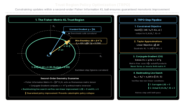
TRPO guarantees stable, monotonic policy improvement by constraining policy parameter updates within a Fisher-information KL divergence trust region.

TRPO optimizes surrogate policy advantages subject to a quadratic Fisher-metric KL divergence constraint, solving for natural gradient steps via Conjugate Gradient.

Why Does This Exist?

In classical policy gradient methods (such as REINFORCE or standard Actor-Critic), policies are optimized using standard gradient ascent in Euclidean parameter space:

$\theta_{t+1} = \theta_t + \alpha \nabla_\theta J(\theta)$

This naive first-order update conceals a dangerous mathematical flaw: Euclidean distance in parameter space ( $\|\Delta \theta\|$ ) does not reflect distance in probability distribution space.

Because neural network parameterizations are highly non-linear, a tiny perturbation $\Delta \theta$ in one layer might barely alter action probabilities, while the exact same perturbation in another layer can cause an abrupt probability collapse (e.g., driving a high-probability winning action from $0.95$ down to $0.02$ ).

Once an oversized step ruins a policy, the agent falls off a performance cliff. Because policy gradients depend on data collected by the current policy, an inferior policy collects degenerate trajectories, making recovery impossible and permanently destroying training runs.

Kakade & Langford (2002) and John Schulman et al. (2015) addressed this through Monotonic Improvement Theory. They proved that bounding the Kullback-Leibler (KL) divergence between consecutive policies guarantees that policy performance never degrades. Trust Region Policy Optimization (TRPO) operationalizes this principle by constraining updates within a second-order Fisher-metric trust region ( $\overline{D}_{\text{KL}}(\theta_{\text{old}}, \theta) \le \delta$ ).

By combining quadratic approximations with the Conjugate Gradient algorithm and a backtracking line search, TRPO guarantees stable, monotonic policy improvement without requiring manual learning rate decay.

Think of It Like This

Stepping Along an Icy Mountain Precipice

Imagine navigating a razor-thin mountain ridge shrouded in dense fog, where one false step means plummeting into the abyss.

If you rely on Ordinary Gradient Descent (First-Order): You gauge the local incline with your boots ( $g = \nabla_\theta L$ ). Because you only feel the immediate slope, you take a full two-meter stride in the direction of the incline. But because the icy ridge curves sharply into a vertical cliff just beyond your footing, that uncurved stride launches you over the edge into catastrophic collapse.

With Trust Region Policy Optimization (Second-Order Curvature + Trust Region): Before moving your feet, you plant a calibrated depth-sensing caliper into the ice beneath you to measure the terrain's second-order curvature (the Fisher Information Matrix $H$ ). The instrument computes a protective elliptical boundary representing the exact maximum distance ( $\delta$ ) you can shift your center of gravity before the ice destabilizes.

Using an efficient directional solver (Conjugate Gradient), you compute the exact optimal stride along that curved ellipse ( $x = H^{-1} g, \beta = \sqrt{2\delta / (g^\top x)}$ ).

Finally, before committing your entire body weight, you execute a cautious backtracking line search: you test 100% of the stride, then 50%, then 25%, verifying that your new footing both increases your elevation and remains safely within the trust region boundary.

Where the analogy stops: Mountain fog is physical terrain. In TRPO, the curvature is the Fisher Information Matrix of a deep neural network, measuring sensitivity across continuous probability distributions over states and actions.

How It Actually Works

The Mathematical Mechanism: Constrained Optimization and Conjugate Gradient

TRPO formulates policy improvement as a constrained optimization problem over the surrogate advantage objective:

$\max_\theta L_{\theta_{\text{old}}}(\theta) \doteq \mathbb{E}_{s \sim \rho^{\theta_{\text{old}}}, a \sim \pi_{\theta_{\text{old}}}} \left[ \frac{\pi_\theta(a \mid s)}{\pi_{\theta_{\text{old}}}(a \mid s)} A^{\pi_{\text{old}}}(s, a) \right]$

$\text{subject to } \overline{D}_{\text{KL}}(\theta_{\text{old}}, \theta) \doteq \mathbb{E}_{s \sim \rho^{\theta_{\text{old}}}} \left[ D_{\text{KL}}(\pi_{\theta_{\text{old}}}(\cdot \mid s) \parallel \pi_\theta(\cdot \mid s)) \right] \le \delta$

Where:

$A^{\pi_{\text{old}}}(s, a)$ is the advantage function under the old policy.
$\delta > 0$ is the trust region budget (typically $\delta \in [0.01, 0.05]$ ).
$\overline{D}_{\text{KL}}(\theta_{\text{old}}, \theta)$ is the expected KL divergence across the state visitation distribution.

Taylor Approximations Around $\theta = \theta_{\text{old}}$

Directly solving this non-linear constrained problem is computationally prohibitive. TRPO approximates both terms using Taylor expansions:

Linear approximation of the objective: $L_{\theta_{\text{old}}}(\theta) \approx L(\theta_{\text{old}}) + g^\top (\theta - \theta_{\text{old}})$ Where $g \doteq \left. \nabla_\theta L_{\theta_{\text{old}}}(\theta) \right|_{\theta = \theta_{\text{old}}}$ is the policy gradient.
Quadratic approximation of the KL constraint: Because $\overline{D}_{\text{KL}}(\theta_{\text{old}}, \theta_{\text{old}}) = 0$ and its first derivative at $\theta_{\text{old}}$ is zero: $\overline{D}_{\text{KL}}(\theta_{\text{old}}, \theta) \approx \frac{1}{2} (\theta - \theta_{\text{old}})^\top H (\theta - \theta_{\text{old}})$ Where $H \doteq \left. \nabla_\theta^2 \overline{D}_{\text{KL}}(\theta_{\text{old}}, \theta) \right|_{\theta = \theta_{\text{old}}}$ is the Fisher Information Matrix (FIM).

This yields the quadratic subproblem:

$\max_{\Delta \theta} g^\top \Delta \theta \quad \text{subject to } \frac{1}{2} \Delta \theta^\top H \Delta \theta \le \delta$

The Analytical Natural Gradient Step

Using the method of Lagrange multipliers, the optimal step direction is the Natural Policy Gradient:

$x \doteq H^{-1} g$

And the step magnitude $\beta$ that saturates the trust region boundary ( $\frac{1}{2} (\beta x)^\top H (\beta x) = \delta$ ) is:

$\beta = \sqrt{\frac{2\delta}{x^\top H x}} = \sqrt{\frac{2\delta}{g^\top H^{-1} g}}$

Yielding the full unconstrained step:

$\Delta \theta = \sqrt{\frac{2\delta}{g^\top H^{-1} g}} H^{-1} g$

Matrix-Free Conjugate Gradient

In deep neural networks with $N = 10^5$ parameters, the Fisher matrix $H \in \mathbb{R}^{N \times N}$ requires 40 gigabytes of memory to store, and computing $H^{-1}$ directly takes $O(N^3)$ operations.

TRPO bypasses this by solving $H x = g$ using the Conjugate Gradient (CG) algorithm. CG requires only computing Hessian-vector products $H v$ , which can be evaluated without ever materializing $H$ :

$H v = \nabla_\theta \left( \left( \nabla_\theta \overline{D}_{\text{KL}} \right)^\top v \right)$

This product is computed using two standard backward passes via automatic differentiation in $O(N)$ time.

Backtracking Line Search

Because the linear objective and quadratic constraint are local approximations, the analytical step $\Delta \theta$ could violate the true non-linear KL constraint or fail to improve the actual surrogate objective.

TRPO executes a backtracking line search along the trajectory:

$\theta_{k+1} = \theta_{\text{old}} + \alpha^j \Delta \theta, \quad j \in \{0, 1, 2, \dots\}$

Where $\alpha \in (0, 1)$ (commonly $\alpha = 0.5$ ). The algorithm selects the first step $j$ satisfying two conditions:

Surrogate Advantage Improvement: $L_{\theta_{\text{old}}}(\theta_{k+1}) \ge 0$
KL Trust Region Compliance: $\overline{D}_{\text{KL}}(\theta_{\text{old}}, \theta_{k+1}) \le \delta$

If no step satisfies these criteria within a maximum number of backtracking trials, the update is rejected, and parameters remain at $\theta_{\text{old}}$ .

Worked Numerical Example

Consider a 2D parameter space $\theta = [\theta_1, \theta_2]^\top$ :

Policy gradient vector: $g = [1.0, 2.0]^\top$
Diagonal Fisher Information Matrix: $H = \begin{bmatrix} 2.0 & 0.0 \\ 0.0 & 4.0 \end{bmatrix}$
Trust region budget: $\delta = 0.05$

(Notice that $H_{22} = 4.0 > H_{11} = 2.0$ , meaning parameter $\theta_2$ alters policy probabilities twice as sensitively as $\theta_1$ .)

Step 1: Solve for Natural Gradient Direction $x = H^{-1} g$

The inverse Fisher matrix is: $H^{-1} = \begin{bmatrix} 0.5 & 0.0 \\ 0.0 & 0.25 \end{bmatrix}$

Computing the natural gradient direction: $x = H^{-1} g = \begin{bmatrix} 0.5 \times 1.0 \\ 0.25 \times 2.0 \end{bmatrix} = \begin{bmatrix} 0.5000 \\ 0.5000 \end{bmatrix}$

Notice how the standard gradient $g = [1.0, 2.0]^\top$ pushed twice as hard along $\theta_2$ , but the Fisher metric equalized the step to $[0.5, 0.5]^\top$ because $\theta_2$ has higher probability curvature.

Step 2: Compute Quadratic Form $g^\top H^{-1} g$

$g^\top x = g^\top H^{-1} g = (1.0 \times 0.5000) + (2.0 \times 0.5000) = 0.5000 + 1.0000 = 1.5000$

Step 3: Compute Maximum Step Scale $\beta$

$\beta = \sqrt{\frac{2\delta}{g^\top H^{-1} g}} = \sqrt{\frac{2(0.05)}{1.5000}} = \sqrt{\frac{0.10}{1.5000}} = \sqrt{\frac{1}{15}} \approx 0.2582$

Step 4: Compute Full Proposed Parameter Step $\Delta \theta$

$\Delta \theta = \beta \cdot x = 0.2582 \times \begin{bmatrix} 0.5000 \\ 0.5000 \end{bmatrix} = \begin{bmatrix} 0.1291 \\ 0.1291 \end{bmatrix}$

Step 5: Exact KL Divergence Verification

Evaluate the quadratic KL divergence: $\overline{D}_{\text{KL}} \approx \frac{1}{2} \Delta \theta^\top H \Delta \theta = \frac{1}{2} \left( 2.0 \times (0.129099)^2 + 4.0 \times (0.129099)^2 \right)$ $\overline{D}_{\text{KL}} = \frac{1}{2} \left( 6.0 \times 0.016667 \right) = \frac{1}{2} (0.1000) = 0.0500 = \delta$

The step lands exactly on the boundary of the trust region.

Step 6: Expected Surrogate Improvement

$\Delta L \approx g^\top \Delta \theta = (1.0 \times 0.1291) + (2.0 \times 0.1291) = 0.3873 > 0$

The expected surrogate objective improves by $+0.3873$ . Because both criteria pass, the backtracking search accepts the step on its first trial ( $j=0$ ).

Code

1import math2from typing import Callable, List, Sequence, Tuple3
4
5def conjugate_gradient(6    h_dot_v: Callable[[Sequence[float]], List[float]],7    g: Sequence[float],8    max_iters: int = 10,9    tol: float = 1e-10,10) -> List[float]:11    """Solve H * x = g for x using Conjugate Gradient without materializing H."""12    x = [0.0] * len(g)13    r = list(g)  # Residual: r_0 = g - H * x_0 = g14    p = list(r)  # Search direction15    r_dot_r = sum(ri * ri for ri in r)16
17    for _ in range(max_iters):18        if r_dot_r < tol:19            break20
21        hp = h_dot_v(p)22        p_h_p = sum(pi * hpi for pi, hpi in zip(p, hp))23
24        if p_h_p <= 0.0:25            break26
27        alpha = r_dot_r / p_h_p28        for j in range(len(x)):29            x[j] += alpha * p[j]30            r[j] -= alpha * hp[j]31
32        new_r_dot_r = sum(ri * ri for ri in r)33        beta = new_r_dot_r / r_dot_r34        for j in range(len(p)):35            p[j] = r[j] + beta * p[j]36
37        r_dot_r = new_r_dot_r38
39    return x40
41
42def compute_trpo_step(43    g: Sequence[float],44    h_dot_v: Callable[[Sequence[float]], List[float]],45    delta: float = 0.05,46    cg_iters: int = 10,47) -> Tuple[List[float], float, float]:48    """Compute the analytical TRPO parameter step Delta theta.49
50    Returns:51        (delta_theta, beta, expected_kl)52    """53    # 1. Solve H * x = g via Conjugate Gradient54    x = conjugate_gradient(h_dot_v, g, max_iters=cg_iters)55
56    # 2. Quadratic curvature form: g^T * H^-1 * g57    g_dot_x = sum(gi * xi for gi, xi in zip(g, x))58    if g_dot_x <= 0.0:59        raise ValueError("Curvature form g^T H^-1 g must be positive.")60
61    # 3. Step scale beta = sqrt(2 * delta / (g^T H^-1 g))62    beta = math.sqrt(2.0 * delta / g_dot_x)63
64    # 4. Full step Delta theta = beta * x65    delta_theta = [beta * xi for xi in x]66
67    # 5. Theoretical quadratic KL divergence68    h_delta_theta = h_dot_v(delta_theta)69    expected_kl = 0.5 * sum(d * hd for d, hd in zip(delta_theta, h_delta_theta))70
71    return delta_theta, beta, expected_kl72
73
74if __name__ == "__main__":75    # Reproduce the exact worked numerical example76    grad_g = [1.0, 2.0]77    fisher_diag = [2.0, 4.0]78    trust_budget_delta = 0.0579
80    def hessian_vector_product(v: Sequence[float]) -> List[float]:81        """Matrix-free product H * v for diagonal Fisher matrix diag(2.0, 4.0)."""82        return [fisher_diag[i] * v[i] for i in range(len(v))]83
84    # Compute step85    step, scale, kl = compute_trpo_step(86        g=grad_g,87        h_dot_v=hessian_vector_product,88        delta=trust_budget_delta,89        cg_iters=2,90    )91
92    surrogate_gain = sum(gi * di for gi, di in zip(grad_g, step))93
94    print(f"Policy Gradient g: {grad_g}")95    print(f"Step Scale beta:   {scale:.4f}")96    print(f"Full Step Delta theta: [d1={step[0]:.4f}, d2={step[1]:.4f}]")97    print(f"Verified KL Divergence: {kl:.6f} (Budget delta={trust_budget_delta})")98    print(f"Surrogate Advantage Gain: {surrogate_gain:.4f}")

1# Expected Output:2# Policy Gradient g: [1.0, 2.0]3# Step Scale beta:   0.25824# Full Step Delta theta: [d1=0.1291, d2=0.1291]5# Verified KL Divergence: 0.050000 (Budget delta=0.05)6# Surrogate Advantage Gain: 0.3873

Watch Out For

The Computational Complexity and Scalability Bottleneck

While TRPO guarantees monotonic policy improvement mathematically, practitioners widely transitioned to Proximal Policy Optimization (PPO) due to three severe operational bottlenecks:

High Wall-Clock Latency: Solving for $H^{-1} g$ requires 10 to 15 Conjugate Gradient iterations. Each CG iteration requires computing a fresh Hessian-vector product ( $H v$ ) via automatic differentiation. Following CG, backtracking line search requires multiple forward evaluations across the entire rollout batch. This makes each TRPO iteration substantially slower than standard stochastic gradient descent.
Incompatibility with Joint Actor-Critic Architectures: The Fisher Information Matrix is defined strictly over the actor's action probability distribution $\pi_\theta(a \mid s)$ . Because value functions $V_\phi(s)$ do not generate probability distributions, TRPO cannot naturally optimize shared actor-critic representations within a single unified loss function.
Complex Distributed Scaling: Hessian-vector products and backtracking line search synchronization do not parallelize cleanly across distributed multi-GPU clusters.

The Fix: Use PPO (Proximal Policy Optimization) for deep reinforcement learning applications. PPO replaces the second-order Fisher constraint and Conjugate Gradient machinery with a first-order clipped surrogate objective ( $L^{\text{CLIP}}$ ), achieving comparable stability and monotonic improvement while running on standard first-order Adam optimizers.

The Quick Version

Solves the Cliff Problem: Constrains policy updates within an explicit probability-space trust region ( $\overline{D}_{\text{KL}} \le \delta$ ), preventing destructive oversized updates that cause irreversible policy collapse.
Fisher Metric Curvature: Scales updates using the Fisher Information Matrix $H$ , accounting for the non-linear Riemannian geometry of probability distributions rather than arbitrary parameter magnitudes.
Matrix-Free Optimization: Employs the Conjugate Gradient algorithm to compute the natural gradient direction $x = H^{-1} g$ in $O(N)$ time using Hessian-vector products, avoiding $O(N^3)$ matrix inversion.
Backtracking Safety Net: Validates candidate updates against both surrogate advantage improvement and the true non-linear KL constraint before committing parameter changes.