Actor-Critic Architecture

Why Does This Exist?

Pure policy gradient methods like REINFORCE suffer from excessive variance because they evaluate actions using complete trajectory returns $G_t = \sum \gamma^k R_{t+k+1}$. In long-horizon tasks, small variations in environment randomness thousands of steps downstream corrupt the gradient of an action taken at step zero. Conversely, pure value-based methods like Q-learning bootstrap efficiently on single-step transitions but cannot natively parameterize continuous action spaces or learn stochastic policies.

The Actor-Critic architecture unites both families into a single hybrid system. An Actor parameterizes the policy $\pi_\theta(a \mid s)$, while a Critic parameterizes a value function $V_\phi(s)$.

Instead of waiting for an entire episode to finish, the Actor updates after every transition (or over small $n$-step rollout windows) using temporal difference (TD) errors provided by the Critic. By replacing the noisy Monte Carlo return $G_t$ with a 1-step bootstrapped estimate $R_{t+1} + \gamma V_\phi(S_{t+1})$, Actor-Critic methods drastically slash variance while retaining the ability to optimize arbitrary continuous or discrete policies.

Think of It Like This

How It Actually Works

Advantage Estimation and Dual Objective Updates

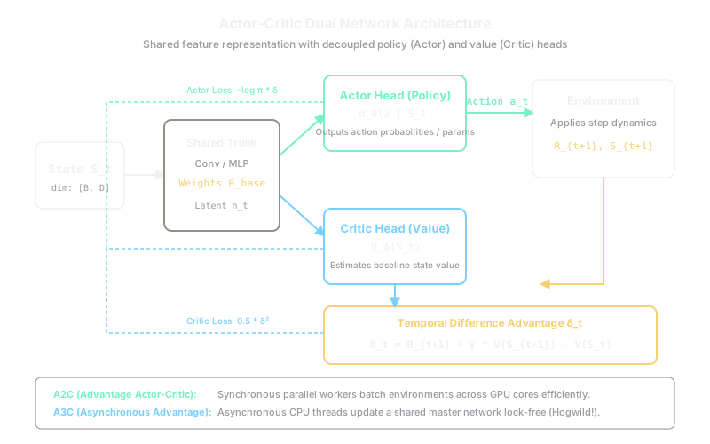
In modern deep Actor-Critic architectures, the Actor and Critic typically share a common convolutional or transformer representation backbone $h_t = f_{\text{base}}(S_t; \theta_{\text{base}})$, branching into two output heads:

1. Actor Head: Outputs action distribution parameters $\pi_\theta(a \mid S_t)$ (e.g., categorical logits or Gaussian mean and standard deviation).
2. Critic Head: Outputs a scalar state-value baseline $V_\phi(S_t) \in \mathbb{R}$.

When the agent executes action $A_t \sim \pi_\theta(\cdot \mid S_t)$, receives reward $R_{t+1}$, and transitions to $S_{t+1}$, the Critic computes the 1-step Temporal Difference Advantage $\delta_t$:

The scalar $\delta_t$ serves as an unbiased estimate of the Advantage function $A(S_t, A_t) = Q(S_t, A_t) - V(S_t)$.

Joint Optimization Objectives

The network parameters are trained jointly using a multi-task composite loss function:

Where:

• Actor Loss: Policy gradient weighted by the advantage: $$\mathcal{L}_{\text{actor}}(\theta) = - \log \pi_\theta(A_t \mid S_t) \, \delta_t$$
• Critic Loss: Mean squared error between predicted value and bootstrapped target: $$\mathcal{L}_{\text{critic}}(\phi) = \frac{1}{2} \left( R_{t+1} + \gamma V_\phi(S_{t+1}) - V_\phi(S_t) \right)^2 = \frac{1}{2} \delta_t^2$$
• Entropy Regularizer: $\mathcal{H}(\pi_\theta) = -\sum_a \pi(a \mid s) \log \pi(a \mid s)$ encourages exploration and prevents premature policy collapse, weighted by coefficient $c_2$.

Coordination Schemes: A2C vs A3C

• A3C (Asynchronous Advantage Actor-Critic): Mnih et al. (2016) introduced asynchronous parallel CPU workers. Multiple environment threads independently step through trajectories and push asynchronous, lock-free gradient updates (Hogwild!) to a centralized global network.
• A2C (Advantage Actor-Critic): Synchronous batched implementation. A centralized coordinator collects fixed-step rollout batches ($n$-steps) across vectorized parallel environments simultaneously, processing them as a single mini-batch on GPU hardware. A2C matches or exceeds A3C's empirical performance without asynchronous stale-gradient artifacts.

Worked Example

An agent observes state $S_0$. The shared network computes:

• Critic evaluation: $V(S_0) = 2.0$
• Actor distribution over two discrete actions: $\pi(a_1 \mid S_0) = 0.70$, $\pi(a_2 \mid S_0) = 0.30$

The agent samples action $A_0 = a_1$. The environment transitions to $S_1$ and awards $R_1 = 1.0$. The Critic evaluates next state: $V(S_1) = 2.5$. Hyperparameters: discount factor $\gamma = 0.9$, learning rate $\alpha = 0.1$.

1. Calculate TD Advantage:

   $$\delta_0 = R_1 + \gamma V(S_1) - V(S_0) = 1.0 + 0.9(2.5) - 2.0 = 1.0 + 2.25 - 2.0 = 1.25$$

   Because $\delta_0 > 0$, taking $a_1$ yielded higher returns than the Critic expected for state $S_0$.

2. Critic Gradient Update:

   $$\text{Target} = R_1 + \gamma V(S_1) = 3.25$$ $$V(S_0) \leftarrow V(S_0) + \alpha \times \delta_0 = 2.0 + 0.1 \times 1.25 = 2.125$$

3. Actor Update Direction:

   • The log-probability of the chosen action $a_1$ is $\log(0.70) \approx -0.3567$.
   • The policy gradient ascends in proportion to $\nabla_\theta \log \pi(a_1 \mid S_0) \times \delta_0 = \nabla_\theta \log \pi(a_1 \mid S_0) \times 1.25$.
   • The probability of taking $a_1$ in $S_0$ will increase on the next training step.

Code

1from typing import Tuple2import numpy as np3
4def compute_actor_critic_step(5    v_current: float,6    v_next: float,7    prob_action: float,8    reward: float,9    gamma: float = 0.9,10    alpha: float = 0.1,11) -> Tuple[float, float, float]:12    """Computes TD advantage and updated state value and policy log-prob delta."""13    # 1-step TD advantage14    td_target = reward + gamma * v_next15    advantage = td_target - v_current16
17    # Critic update: move value toward td_target18    updated_v = v_current + alpha * advantage19
20    # Actor policy gradient step: delta = alpha * (grad_log_pi * advantage)21    # For a softmax logit update, the positive advantage encourages this action22    logit_delta = alpha * advantage23
24    return advantage, updated_v, logit_delta25
26# Test case matching worked example27adv, new_v, delta_logit = compute_actor_critic_step(28    v_current=2.0,29    v_next=2.5,30    prob_action=0.7,31    reward=1.0,32    gamma=0.9,33    alpha=0.1,34)35
36print(f"Advantage (delta): {adv:.2f}")37# -> Advantage (delta): 1.2538
39print(f"Updated V(S0): {new_v:.4f}")40# -> Updated V(S0): 2.125041
42print(f"Actor logit shift: +{delta_logit:.4f}")43# -> Actor logit shift: +0.1250

Watch Out For

The Quick Version

• Actor-Critic algorithms decouple decision-making (Actor $\pi_\theta$) from performance evaluation (Critic $V_\phi$).
• The Critic computes a 1-step temporal difference error $\delta_t = R_{t+1} + \gamma V(S_{t+1}) - V(S_t)$ that acts as a low-variance baseline advantage.
• Synchronous Advantage Actor-Critic (A2C) executes batched environments on GPUs, eliminating the stale-gradient instability of asynchronous A3C.

What to Read Next

• Advanced RL Paradigms
• Offline Reinforcement Learning
• Temporal Difference Learning