Advantages of TD over MC and DP
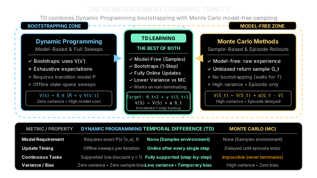
Temporal difference learning bridges the gap between dynamic programming and Monte Carlo methods by combining model-free experience sampling with immediate one-step bootstrapping. This allows agents to learn online from incomplete episodes with significantly lower variance.
Why Does This Exist?
In reinforcement learning, estimating how good a state is—its value —requires predicting cumulative future rewards. Before Temporal Difference (TD) learning emerged, practitioners relied on two classical frameworks, each suffering from a crippling limitation:
- Dynamic Programming (DP) requires a complete model: DP methods like policy iteration and value iteration compute values by calculating expected future rewards. However, they require perfect mathematical specifications of transition probabilities and reward distributions. In complex domains such as robotic locomotion, autonomous navigation, or game playing, writing down these transition matrices is impossible. Furthermore, DP requires exhaustive sweeps over all states, making it intractable for large state spaces.
- Monte Carlo (MC) requires complete episodes and suffers from high variance: MC methods eliminate the need for an environmental model by interacting with the world and sampling raw trajectories. But MC updates only after an episode terminates, because it computes the actual total return . This means MC cannot learn on continuous, non-terminating tasks. Moreover, summing rewards over an entire rollout compounds the stochastic randomness of every subsequent transition and action, producing high-variance targets that require vast amounts of data to converge.
Temporal Difference learning resolves both bottlenecks simultaneously. Like Monte Carlo, TD is model-free, learning directly from sampled transitions without knowing transition probabilities. Like Dynamic Programming, TD bootstraps, updating value estimates based on other learned value estimates after a single transition. This synthesis gives TD the sample efficiency of online learning, the low variance of one-step updates, and the universal ability to learn from continuing tasks.
Think of It Like This
Predicting Your Evening Commute
Imagine you leave your office at 5:00 PM and want to estimate how many minutes your drive home will take.
- The Dynamic Programming Approach: Before turning your car's key, a citywide supercomputer runs a comprehensive traffic simulation of every intersection, green light timing, pedestrian crosswalk, and driver in the city to compute your exact expected travel time. If you do not possess a flawless simulation of the entire road network, you cannot even begin your calculation.
- The Monte Carlo Approach: You depart expecting a 45-minute trip. Fifteen minutes in, you hit a standstill gridlock on the highway. Under pure Monte Carlo rules, you are forbidden from updating your commute prediction while stuck. You must finish the journey, park in your driveway at 6:30 PM (90 minutes total), look at your watch, and only then update your departure estimate. Even worse, if you were on an endless road trip with no final destination, you would never update at all.
- The Temporal Difference Approach: At 5:15 PM, when you hit the gridlock, your remaining travel estimate suddenly jumps from 30 minutes to 60 minutes. Under TD learning, you adjust your departure estimate immediately at minute 15: your expectation updates on the fly from 45 minutes to 75 minutes based on the local shift in estimates. You do not wait to arrive home to learn from the delay.
Where the analogy breaks down: Commute times in human life rely on subjective intuition and visual road signs. TD learning mathematically updates scalar value functions over discounted Markovian reward streams via the Bellman operator. Furthermore, in early learning iterations, your remaining travel estimates may be wrong, temporarily biasing your initial TD updates until those downstream estimates mature.
How It Actually Works
The Reinforcement Learning Trinity: DP, MC, and TD
The relationship between Dynamic Programming, Monte Carlo, and Temporal Difference learning is characterized by two orthogonal dimensions: sampling (whether the algorithm requires an environmental model or learns from experience) and bootstrapping (whether updates rely on successor value estimates or complete episode returns).
BOOTSTRAPPING (Depth = 1) ▲ │ Dynamic │ Temporal Programming │ Difference [TD(0)] (DP) │ │ EXHAUSTIVE ◄─────────────────┼─────────────────► SAMPLING EXPECTATIONS │ EXPERIENCE (Model-Based) │ (Model-Free) │ │ Monte Carlo │ (MC) ▼ FULL ROLLOUT (Depth = ∞)1. Dynamic Programming Backup (Model-Based, Bootstrapping)
Dynamic Programming performs full-width, shallow-depth backups using the Bellman expectation equation:
- Model dependency: Requires the transition probability function .
- Bootstrapping: Yes, uses current estimates .
- Sampling: No, computes expectations across all possible next states.
- Variance: Zero (deterministic calculation under a known model).
2. Monte Carlo Backup (Model-Free, No Bootstrapping)
Monte Carlo samples individual trajectories and updates values toward the full discounted empirical return :
where the return is defined across the entire remaining trajectory until terminal time step :
- Model dependency: None (model-free).
- Bootstrapping: No, relies exclusively on realized rewards.
- Sampling: Yes, follows sample paths through the environment.
- Variance: High, because stochastic state transitions and action choices compound multiplicatively along the path.
- Bias: Zero, because .
3. Temporal Difference TD(0) Backup (Model-Free, Bootstrapping)
TD(0) samples a single step and bootstraps using the successor state estimate :
The quantity in brackets is the TD error, denoted :
where the TD target is .
- Model dependency: None (model-free).
- Bootstrapping: Yes, updates toward an estimate rather than the true return .
- Sampling: Yes, updates along experienced state-action transitions.
- Variance: Low, because the target depends only on the single immediate reward and the smooth value .
- Bias: Initial bias exists due to imperfect estimates, but bias vanishes asymptotically as values converge.
Feature Comparison Matrix
| Property | Dynamic Programming (DP) | Monte Carlo (MC) | Temporal Difference (TD) |
|---|---|---|---|
| Model Required | Complete model | None (Model-Free) | None (Model-Free) |
| Bootstrapping | Yes (depth 1) | No (depth ) | Yes (depth 1) |
| Sampling | Exhaustive expectation | Sample trajectories | Sample transitions |
| Update Timing | Offline batch sweeps | Delayed until episode ends | Online after every step |
| Continuous Tasks | Supported | Impossible (requires termination) | Fully supported |
| Target Variance | Zero | High (accumulates trajectory noise) | Low (single-step noise) |
| Estimation Bias | Zero (with true model) | Unbiased | Biased initially, vanishes asymptotically |
| Computation per Step | at episode boundary | constant time |
Worked numerical example
Consider a 3-state chain environment with states leading to a terminal state:
Let the discount factor be and the learning rate be . Suppose the current value estimates are:
Step 1: The 1-Step TD Update (Online at )
After taking action in , the agent receives immediate reward and transitions to . The agent computes the TD target and TD error immediately:
The value of updates right away:
Notice: State is updated at time step 1. The agent did not need to know what happens at , , or whether the episode ever finishes.
Step 2: The Monte Carlo Update (Delayed until )
Under Monte Carlo, no update can occur until the agent traverses and and lands in the terminal state at . Only then can it compute the full discounted return :
The MC update for occurs only at the end of the episode:
Why This Difference Matters
- Information propagation: TD began improving its estimate of at . In long or continuous environments, TD propagates value information backward step by step during the rollout.
- Variance isolation: If the final transition from had a noisy reward (e.g., half the time and half the time), every MC return would swing wildly. TD replaces the entire downstream tail with , insulating the update of from the variance of subsequent transitions.
Code
The following script benchmarks TD(0) against First-Visit Monte Carlo on a 5-state Random Walk. It quantifies target variance and convergence speed:
import mathimport randomimport statisticsfrom typing import Dict, List, Tuple
def compare_td_and_mc() -> None: # Set seed for exact numerical reproducibility random.seed(42)
# 5-State Random Walk: states 1..5; terminals 0 (reward 0) and 6 (reward 1) # Analytical true values: V*(s) = s / 6.0 true_v: Dict[int, float] = {s: s / 6.0 for s in range(1, 6)}
def generate_episode() -> List[Tuple[int, float, int]]: trajectory: List[Tuple[int, float, int]] = [] state = 3 # Start in the center state while state not in (0, 6): action = -1 if random.random() < 0.5 else 1 next_state = state + action reward = 1.0 if next_state == 6 else 0.0 trajectory.append((state, reward, next_state)) state = next_state return trajectory
# Generate 150 shared episodes for identical empirical conditions episodes: List[List[Tuple[int, float, int]]] = [ generate_episode() for _ in range(150) ]
# 1. Target Variance Comparison at Center State (S3) # Compare empirical variance of MC return G vs TD target (R + gamma * V(s')) mc_returns_s3: List[float] = [] td_targets_s3: List[float] = [] baseline_v: Dict[int, float] = {s: s / 6.0 for s in range(7)}
for ep in episodes: for i, (s, r, s_next) in enumerate(ep): if s == 3: # TD target uses single-step reward + successor estimate td_targets_s3.append(r + 1.0 * baseline_v[s_next]) # MC return sums all future rewards along the trajectory return_g = sum(step[1] for step in ep[i:]) mc_returns_s3.append(return_g) break
var_mc = statistics.variance(mc_returns_s3) var_td = statistics.variance(td_targets_s3)
# 2. Value Estimation Convergence (TD(0) vs First-Visit MC) v_mc: Dict[int, float] = {s: 0.5 for s in range(1, 6)} v_td: Dict[int, float] = {s: 0.5 for s in range(1, 6)} alpha = 0.05
for ep in episodes: # First-Visit MC update (delayed until episode completion) visited_states = set() accumulated_g = 0.0 for s, r, _ in reversed(ep): accumulated_g += r if s not in visited_states: visited_states.add(s) v_mc[s] += alpha * (accumulated_g - v_mc[s])
# TD(0) update (applied online after every single transition) for s, r, s_next in ep: next_val = 0.0 if s_next in (0, 6) else v_td[s_next] td_target = r + 1.0 * next_val v_td[s] += alpha * (td_target - v_td[s])
rmse_mc = math.sqrt(sum((v_mc[s] - true_v[s]) ** 2 for s in range(1, 6)) / 5) rmse_td = math.sqrt(sum((v_td[s] - true_v[s]) ** 2 for s in range(1, 6)) / 5)
print(f"MC Target Variance (S3): {var_mc:.4f}") print(f"TD Target Variance (S3): {var_td:.4f}") print(f"MC RMSE after 150 episodes: {rmse_mc:.4f}") print(f"TD RMSE after 150 episodes: {rmse_td:.4f}")
compare_td_and_mc()
# -> Expected output:# -> MC Target Variance (S3): 0.2501# -> TD Target Variance (S3): 0.0280# -> MC RMSE after 150 episodes: 0.0611# -> TD RMSE after 150 episodes: 0.0464Watch Out For
Initial Estimation Bias and the Deadly Triad
While bootstrapping drastically reduces variance, it introduces estimation bias. Because the TD target uses the agent's current estimate , any inaccuracies in pollute the update to .
The Symptom: In tabular settings, TD converges to the true value function despite this bias (given standard Robbins-Monro step-size decays ). However, in deep reinforcement learning, bootstrapping interacts destructively with two other design choices to form the Deadly Triad:
- Function Approximation: Using non-linear neural networks to represent values.
- Bootstrapping: Updating estimates based on downstream learned estimates.
- Off-Policy Learning: Updating target policies from replay buffers or alternative behavioral policies.
When all three elements are present, bootstrapping errors amplify iteratively, leading to catastrophic value divergence and unbounded Q-value overestimation.
The Fix:
- In tabular and linear settings, set step sizes conservatively () to allow bootstrapping noise to average out smoothly.
- In deep RL, decouple the update target from the parameters being optimized using target networks (updated periodically or via Polyak averaging) and double Q-learning to suppress target overestimation.
- When variance permits, use multi-step TD() or TD() to blend the low-bias benefits of Monte Carlo rollouts with the low-variance benefits of bootstrapping.
The Quick Version
- The Best of Both Worlds: Temporal Difference learning combines the model-free interaction of Monte Carlo with the one-step bootstrapping of Dynamic Programming.
- No Environmental Model Needed: Unlike Dynamic Programming, TD does not require explicit transition probability matrices or reward functions; it learns directly from experienced transitions.
- Online, Step-by-Step Updates: Unlike Monte Carlo, TD updates immediately after each transition, enabling efficient learning in real time and supporting non-terminating, continuous environments.
- Lower Target Variance: Bootstrapping on avoids accumulating the stochastic noise of entire future trajectories, allowing TD to converge with significantly fewer training samples than Monte Carlo.