Dynamic Programming in RL

Dynamic programming computes optimal policies by breaking sequential decisions into overlapping subproblems and bootstrapping value estimates using a complete mathematical model of the environment.

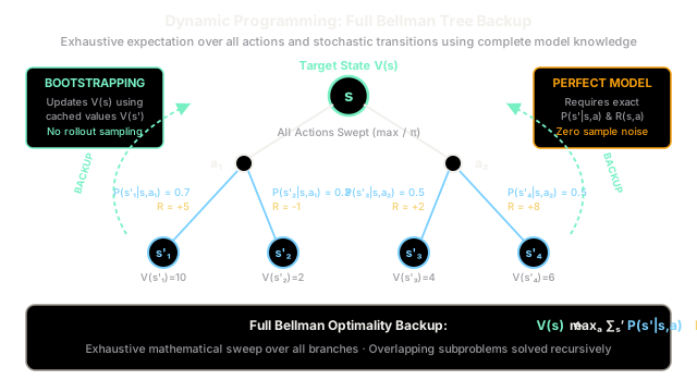
Dynamic programming computes exact value functions by executing full Bellman backups across all candidate actions and transition probabilities using complete model dynamics.

Why Does This Exist?

In sequential decision-making, an agent aims to choose actions that maximize cumulative rewards over an extended or infinite horizon. A naive search over all possible future action sequences explodes exponentially with time: an agent planning $T$ steps ahead with $|\mathcal{A}|$ available actions must evaluate $|\mathcal{A}|^T$ distinct trajectories. For a modest horizon of $T = 20$ with $4$ actions, this requires comparing over $10^{12}$ distinct paths—an intractable combinatorial explosion.

Richard Bellman resolved this dilemma through the Principle of Optimality: an optimal policy has the property that whatever the initial state and initial decision are, the remaining decisions must constitute an optimal policy with regard to the state resulting from the first decision. Because sequential decisions satisfy recursive subproblem overlap, the global optimization problem can be decomposed into local, one-step subproblems.

Dynamic Programming (DP) provides the collection of algorithms that solve Markov Decision Processes by turning Bellman equations into iterative assignment updates. Unlike model-free reinforcement learning methods—such as Temporal Difference Learning or Monte Carlo Methods—which must sample transitions through trial-and-error interaction, DP operates as a planning framework. It assumes a perfect mathematical model of the environment's physics and reward mechanics, executing exhaustive expectations across all possible outcomes. This eliminates sample variance entirely and forms the theoretical backbone for Value Functions and policy optimization.

Think of It Like This

GPS route recalculation with a preloaded city blueprint

Imagine an advanced satellite navigation computer preloaded with a centimeter-accurate offline blueprint of every street, intersection, turn restriction, and statistical traffic delay in a metropolis.

You are sitting at an intersection ( $s$ ) wanting the fastest route to the central railway station. The GPS does not need to dispatch physical test vehicles into random alleys to find out where they lead—an approach analogous to trial-and-error model-free exploration. Because it holds the complete map graph and travel cost tables ( $P(s' \mid s, a)$ and $R(s, a)$ ), it computes the optimal journey offline.

If the GPS already knows the estimated travel time from every adjacent intersection ( $s'$ ) to the destination, recalculating the optimal decision at intersection $s$ requires looking only one step ahead:

Examine each available street you could take ( $a$ ).
Factor in the expected delay on that specific street segment ( $R$ ).
Add the precomputed travel duration from the destination intersection onward ( $V(s')$ ).
Select the turn with the minimum total expected time.

By caching and iteratively updating the travel times of neighboring intersections, the system solves the global navigation problem without simulating endless full routes.

Where the analogy stops: Standard road navigation maps are largely deterministic—turning left onto Main Street lands you on Main Street with certainty. In reinforcement learning MDPs, DP explicitly computes expectations over stochastic environments where turning onto an icy street might skid you into several alternative intersections with known probabilities ( $P(s' \mid s, a)$ ).

How It Actually Works

Bellman Backup Operators and Mathematical Formulation

Dynamic programming requires complete access to the four-tuple transition dynamics of a finite Markov Decision Process:

$\mathcal{S}$ : The set of all valid states.
$\mathcal{A}$ : The set of all possible actions.
$P(s' \mid s, a) = \Pr(S_{t+1} = s' \mid S_t = s, A_t = a)$ : The transition probability kernel.
$R(s, a, s')$ : The immediate scalar reward received after transitioning from $s$ to $s'$ under action $a$ .
$\gamma \in [0, 1)$ : The discount factor ensuring convergence over infinite horizons.

The expected reward for taking action $a$ in state $s$ is formalized as:

$R(s, a) = \sum_{s' \in \mathcal{S}} P(s' \mid s, a) R(s, a, s')$

The Bootstrap Principle

Dynamic programming updates its value estimates based on other value estimates. Rather than waiting until the end of an episode to compute empirical returns (as in Monte Carlo rollouts), DP performs bootstrapping: it truncates the horizon after a single step and substitutes the current cached value estimate $V(s')$ for the remainder of the trajectory.

Bellman Expectation Backup Operator ( $T^\pi$ )

For a fixed policy $\pi(a \mid s)$ , the value function satisfies the linear system known as the Bellman expectation equation. In DP, this equation is turned into an operational update operator $T^\pi$ :

$(T^\pi V)(s) \doteq \sum_{a \in \mathcal{A}} \pi(a \mid s) \sum_{s' \in \mathcal{S}} P(s' \mid s, a) \left[ R(s, a, s') + \gamma V(s') \right]$

Iterative policy evaluation repeatedly applies this operator: $V_{k+1} = T^\pi V_k$ .

Bellman Optimality Backup Operator ( $T^*$ )

To identify the optimal policy $\pi^*$ , the Bellman optimality backup operator $T^*$ performs a greedy maximization over all available actions:

$(T^* V)(s) \doteq \max_{a \in \mathcal{A}} \sum_{s' \in \mathcal{S}} P(s' \mid s, a) \left[ R(s, a, s') + \gamma V(s') \right]$

Equivalently, in terms of state-action values $Q(s, a)$ :

$(T^* Q)(s, a) \doteq \sum_{s' \in \mathcal{S}} P(s' \mid s, a) \left[ R(s, a, s') + \gamma \max_{a' \in \mathcal{A}} Q(s', a') \right]$

Contraction Mapping and Guaranteed Convergence

A critical property of the dynamic programming operators is that both $T^\pi$ and $T^*$ are $\gamma$ -contraction mappings in the supremum norm ( $\|V\|_\infty = \max_{s \in \mathcal{S}} |V(s)|$ ):

$\|T^* U - T^* V\|_\infty \le \gamma \|U - V\|_\infty \quad \text{for all } U, V \in \mathbb{R}^{|\mathcal{S}|}$

Because $\gamma < 1$ , Banach's Fixed-Point Theorem guarantees that:

A unique optimal fixed point $V^*$ exists such that $T^* V^* = V^*$ .
Repeated application $V_{k+1} = T^* V_k$ converges exponentially to $V^*$ from any arbitrary initial vector $V_0$ .

Dynamic programming organizes these backups into two canonical algorithmic paradigms:

Policy Iteration: Alternates between exhaustive policy evaluation (solving for $V^\pi$ ) and greedy policy improvement ( $\pi'(s) = \arg\max_a Q^\pi(s, a)$ ).
Value Iteration: Applies the optimality operator $T^*$ directly across all states in each sweep, interleaving policy evaluation and improvement into a single step.

Worked numerical example

Consider an agent in target state $s$ with discount factor $\gamma = 0.9$ . The agent has two candidate actions: $a_1$ and $a_2$ .

The environment dynamics model defines the following branches:

Action $a_1$ (stochastic with two successor states $s'_1$ $s_{1}^{'}$ and $s'_2$ $s_{2}^{'}$ ):
- Transition to $s'_1$ : probability $P(s'_1 \mid s, a_1) = 0.8$ , immediate reward $R(s, a_1, s'_1) = +2.0$ , cached estimate $V_k(s'_1) = 10.0$ .
- Transition to $s'_2$ : probability $P(s'_2 \mid s, a_1) = 0.2$ , immediate reward $R(s, a_1, s'_2) = +5.0$ , cached estimate $V_k(s'_2) = 4.0$ .
Action $a_2$ (deterministic transition to successor state $s'_3$ $s_{3}^{'}$ ):
- Transition to $s'_3$ : probability $P(s'_3 \mid s, a_2) = 1.0$ , immediate reward $R(s, a_2, s'_3) = +1.0$ , cached estimate $V_k(s'_3) = 9.0$ .

Step 1: Compute discounted branch targets for action $a_1$

For each successor state $s'$ , compute the one-step target $R(s, a_1, s') + \gamma V_k(s')$ :

Target for branch $s'_1$ : $G_1 = 2.0 + 0.9 \times 10.0 = 2.0 + 9.0 = 11.0$
Target for branch $s'_2$ : $G_2 = 5.0 + 0.9 \times 4.0 = 5.0 + 3.6 = 8.6$

Step 2: Compute the expectation for action $a_1$ (Action-Value $Q(s, a_1)$ )

Apply the probability-weighted Bellman expectation across both branches: $Q_k(s, a_1) = P(s'_1 \mid s, a_1) \cdot G_1 + P(s'_2 \mid s, a_1) \cdot G_2$ $Q_k(s, a_1) = (0.8 \times 11.0) + (0.2 \times 8.6) = 8.80 + 1.72 = 10.52$

Step 3: Compute the expectation for action $a_2$ (Action-Value $Q(s, a_2)$ )

Compute the one-step target for the deterministic branch: $Q_k(s, a_2) = 1.0 \times \left[ 1.0 + 0.9 \times 9.0 \right] = 1.0 + 8.10 = 9.10$

Step 4: Apply the Bellman Optimality Backup Operator

The Bellman optimality operator selects the maximum value among all actions: $V_{k+1}(s) = \max \left\{ Q_k(s, a_1), Q_k(s, a_2) \right\} = \max \{ 10.52, 9.10 \} = 10.52$

The derived greedy policy for state $s$ selects: $\pi_{k+1}(s) = \arg\max_{a} Q_k(s, a) = a_1$

The value of state $s$ has been updated from its prior value to $10.52$ purely by backing up expectations from cached successor state estimates and the known transition model.

Code

1from dataclasses import dataclass2from typing import Dict, List, Tuple3
4
5@dataclass(frozen=True)6class Transition:7    """Represents a stochastic branch in the environment dynamics model."""8    prob: float        # P(s' | s, a)9    next_state: str    # Successor state s'10    reward: float      # Immediate reward R(s, a, s')11
12
13class ModelMDP:14    """Tabular Markov Decision Process solved via Dynamic Programming backups."""15
16    def __init__(17        self,18        states: List[str],19        actions: List[str],20        transitions: Dict[Tuple[str, str], List[Transition]],21        gamma: float = 0.9,22    ) -> None:23        self.states = states24        self.actions = actions25        self.transitions = transitions26        self.gamma = gamma27
28    def compute_q_value(29        self, state: str, action: str, value_function: Dict[str, float]30    ) -> float:31        """32        Computes Q(s, a) using the full Bellman expectation backup:33        Q(s, a) = sum_{s'} P(s'|s,a) * [ R(s,a,s') + gamma * V(s') ]34        """35        branches = self.transitions.get((state, action), [])36        if not branches:37            return 0.038
39        q_val = 0.040        for branch in branches:41            discounted_future = self.gamma * value_function[branch.next_state]42            q_val += branch.prob * (branch.reward + discounted_future)43        return q_val44
45    def bellman_optimality_backup(46        self, state: str, value_function: Dict[str, float]47    ) -> Tuple[float, str]:48        """49        Executes a 1-step Bellman Optimality Backup for a single state:50        V(s) <- max_a Q(s, a)51        """52        action_values = {53            action: self.compute_q_value(state, action, value_function)54            for action in self.actions55        }56        best_action = max(action_values, key=lambda a: action_values[a])57        best_value = action_values[best_action]58        return best_value, best_action59
60    def full_sweep_backup(61        self, value_function: Dict[str, float]62    ) -> Tuple[Dict[str, float], Dict[str, str]]:63        """Performs one synchronous dynamic programming sweep across all states."""64        new_v: Dict[str, float] = {}65        greedy_policy: Dict[str, str] = {}66
67        for s in self.states:68            v_val, best_act = self.bellman_optimality_backup(s, value_function)69            new_v[s] = round(v_val, 4)70            greedy_policy[s] = best_act71
72        return new_v, greedy_policy73
74
75if __name__ == "__main__":76    # Define states and actions matching the worked numerical example77    states = ["s", "s'_1", "s'_2", "s'_3"]78    actions = ["action_a", "action_b"]79
80    transitions = {81        ("s", "action_a"): [82            Transition(prob=0.8, next_state="s'_1", reward=2.0),83            Transition(prob=0.2, next_state="s'_2", reward=5.0),84        ],85        ("s", "action_b"): [86            Transition(prob=1.0, next_state="s'_3", reward=1.0),87        ],88        # Terminal successor states with zero rewards89        ("s'_1", "action_a"): [Transition(prob=1.0, next_state="s'_1", reward=0.0)],90        ("s'_1", "action_b"): [Transition(prob=1.0, next_state="s'_1", reward=0.0)],91        ("s'_2", "action_a"): [Transition(prob=1.0, next_state="s'_2", reward=0.0)],92        ("s'_2", "action_b"): [Transition(prob=1.0, next_state="s'_2", reward=0.0)],93        ("s'_3", "action_a"): [Transition(prob=1.0, next_state="s'_3", reward=0.0)],94        ("s'_3", "action_b"): [Transition(prob=1.0, next_state="s'_3", reward=0.0)],95    }96
97    # Initial cached state-value estimates V_k98    v_k = {99        "s": 0.0,100        "s'_1": 10.0,101        "s'_2": 4.0,102        "s'_3": 9.0,103    }104
105    env = ModelMDP(states, actions, transitions, gamma=0.9)106
107    print("--- 1-Step DP Bellman Backup for State 's' ---")108    for act in actions:109        q = env.compute_q_value("s", act, v_k)110        print(f"Q(s, {act}) = {q:.4f}")111
112    new_v_s, best_action = env.bellman_optimality_backup("s", v_k)113    print(f"\nUpdated Value V_{{k+1}}(s) = {new_v_s:.4f}")114    print(f"Greedy Policy pi_{{k+1}}(s)   = '{best_action}'")115
116    # Perform a full-sweep backup across the entire state space117    updated_v, greedy_policy = env.full_sweep_backup(v_k)118    print("\nFull-sweep updated values:", updated_v)119    print("Derived greedy policy:   ", greedy_policy)120
121    # Expected Output:122    # --- 1-Step DP Bellman Backup for State 's' ---123    # Q(s, action_a) = 10.5200124    # Q(s, action_b) = 9.1000125    #126    # Updated Value V_{k+1}(s) = 10.5200127    # Greedy Policy pi_{k+1}(s)   = 'action_a'128    #129    # Full-sweep updated values: {'s': 10.52, "s'_1": 9.0, "s'_2": 3.6, "s'_3": 8.1}130    # Derived greedy policy:    {'s': 'action_a', "s'_1": 'action_a', "s'_2": 'action_a', "s'_3": 'action_a'}

Watch Out For

The fatal dependency on a perfect environment model

Dynamic programming is fundamentally a planning algorithm, not a learning algorithm. Its Bellman backup equations require computing the exact mathematical expectation $\sum_{s'} P(s' \mid s, a) [\dots]$ . If transition probabilities $P(s' \mid s, a)$ or reward dynamics $R(s, a, s')$ are unknown, noisy, or non-stationary, pure DP cannot execute a single step.

In practical real-world problems like robotics or stock trading, the environment dynamics cannot be written down in closed form. Practitioners attempting to apply DP in model-free settings face total failure.

The Fix: When the environment is accessible only via interaction samples $(s, a, r, s')$ , use model-free reinforcement learning methods such as Temporal Difference Learning (Q-learning, SARSA) or Monte Carlo Methods. Alternatively, apply Model-Based RL to learn an empirical transition model $\hat{P}(s' \mid s, a)$ before executing DP planning backups.

The curse of dimensionality and state space explosion

A synchronous DP sweep iterates over every state $s \in \mathcal{S}$ and evaluates every action $a \in \mathcal{A}$ across all possible transitions $s'$ . For dense transition models, the computational complexity per sweep is $\mathcal{O}(|\mathcal{S}|^2 |\mathcal{A}|)$ .

While polynomial in the number of states, $|\mathcal{S}|$ grows exponentially with the number of state variables—a barrier Bellman termed the "curse of dimensionality." A robotic arm with 10 continuous joint angles or a game with 30 discrete state attributes has an astronomical state space that exhausts memory and renders tabular DP sweeps impossible.

The Fix: Transition from tabular dynamic programming to Approximate Dynamic Programming (ADP). Replace tabular state arrays with parametric function approximation (such as deep neural networks in Deep Q-Networks and Actor-Critic architectures), or employ asynchronous updates and sample-based tree search (such as Monte Carlo Tree Search) to focus Bellman backups only on trajectories visited by the agent.

The Quick Version

Planning with a perfect model: Dynamic programming solves MDPs by computing exact expectations over fully known transition distributions $P(s' \mid s, a)$ and reward functions $R(s, a)$ , eliminating sample variance.
Bootstrapping via contraction mappings: It avoids exponential trajectory rollouts by recursively updating current state values using cached values of successor states via contraction operators ( $T^\pi$ and $T^*$ ), guaranteeing unique convergence.
Exhaustive backup tree: Unlike sample-based RL which samples single transitions $(s, a, r, s')$ , DP performs full tree backups across every action and every stochastic successor state.
Foundation of modern RL: While tabular DP suffers from the curse of dimensionality in large state spaces, its Bellman backup formulations serve as the mathematical bedrock for policy iteration, value iteration, and deep reinforcement learning.