Monte Carlo Methods

Monte Carlo methods price a state by playing whole episodes from it and averaging what actually came back, with no model and no bootstrapping.

Two finished episodes return 9 and 12 from state A, so its value estimate is the average 10.5 with no model and no bootstrapping

Why Does This Exist?

Pricing a state means answering how much total reward follows from it. Dynamic programming answers exactly but demands the full transition model $P(s' \mid s, a)$ , which real problems rarely provide, plus sweeps over huge state spaces that do not scale.

Monte Carlo methods answer from experience instead. Play an episode to termination, add up the rewards, repeat, average. No model is consulted and no estimate is built on another estimate, so there is no bootstrapping bias to unwind. The law of large numbers does the work: as independent returns accumulate, their average converges to the true expected value. This page covers that prediction mechanism. The counting variants live in first visit versus every visit, the bootstrapping alternative is temporal difference learning, and the control loop on top is Monte Carlo control.

The one idea you need first

The state value $V^{\pi}(s)$ is the expected discounted total from $s$ onward under policy $\pi$ . Value functions define it and its action value sibling $Q$ . Monte Carlo replaces that expectation with a plain average of finished totals.

Think of It Like This

Timing a maze route with a stopwatch

You need the average drive time from an intersection to the maze exit but own no map. So you drive it: first trip takes 9 minutes through the north passage, second takes 12 through the south. Your estimate for that intersection is the average, 10.5 minutes. No map, no traffic model, just finished trips and a mean.

More trips sharpen the number and a detour ridden twice still counts once per trip under first visit rules. Where it stops: traffic is far less random than a stochastic MDP, where whole trajectory randomness inflates the spread of totals and learning needs many more trips.

How It Actually Works

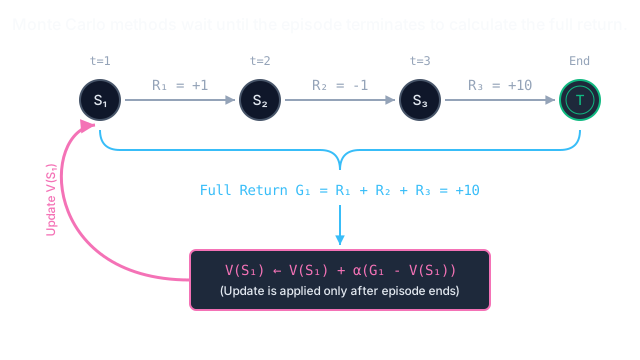
Follow policy $\pi$ until termination to get $S_0, A_0, R_1, \dots, S_T$ . The return from step $t$ is the discounted sum to the end:

G_t = R_{t+1} + \gamma R_{t+2} + \gamma^2 R_{t+3} + \dots + \gamma^{T-t-1} R_T

with discount $\gamma$ in $[0, 1]$ . Then update every visited state with an incremental average over $N(s)$ visits:

V(s) \leftarrow V(s) + \frac{1}{N(s)}[G_t - V(s)]

The update uses the sampled total $G_t$ only, never the current estimate of a successor, which is exactly what non bootstrapping means. When a state appears several times in one episode, first visit uses only the first $G_t$ while every visit uses each one; both converge, with slightly different variance. Episodes must terminate, or $G_t$ never materializes.

Worked example

Price intersection $A$ with $\gamma = 1.0$ from two finished trips. Rewards are written per visited state as (state, reward arriving there):

Episode 1: $(A, 0)$ , $(B, 1)$ , $(C, -2)$ , $(T, 10)$ . Adding the rewards along the trip, the total from $A$ is $0 + 1 - 2 + 10 = 9$ . Episode 2: $(A, 0)$ , $(C, 2)$ , $(T, 10)$ , giving $0 + 2 + 10 = 12$ from $A$ .

Averaging the two first visit totals at $A$ :

V(A) = \frac{9 + 12}{2} = 10.5

Two trips, one addition, one division: the estimate is 10.5 with no model and no bootstrapped value anywhere in the computation.

Code

This snippet implements first visit prediction over the two worked episodes and prints the value of $A$ .

1import numpy as np2
3
4def first_visit_values(episodes: list[list[tuple[str, float]]]) -> dict[str, float]:5    totals: dict[str, list[float]] = {}6    for episode in episodes:7        g = 0.08        seen: set[str] = set()9        for t in range(len(episode) - 1, -1, -1):10            state, reward = episode[t]11            g = g + reward12            earlier = [s for s, _ in episode[:t]]13            if state not in earlier and state not in seen:14                seen.add(state)15                totals.setdefault(state, []).append(g)16    return {s: float(np.mean(v)) for s, v in totals.items()}17
18
19episodes = [20    [("A", 0.0), ("B", 1.0), ("C", -2.0), ("T", 10.0)],21    [("A", 0.0), ("C", 2.0), ("T", 10.0)],22]23values = first_visit_values(episodes)24print(values["A"])  # -> 10.5

The printout is 10.5, matching $(9 + 12) / 2$ from the hand computation. Adding more episodes to the list would keep sharpening every visited state's average.

Watch Out For

Requiring termination in tasks that never end

Monte Carlo waits for the final step before any update, so a continuing task such as an always on controller or a loop that rarely terminates yields no $G_t$ and therefore no learning, while trajectories consume memory without bound.

Symptom: buffers grow, updates never fire, values stay at initialization. Fix: impose a horizon with resets for episodic evaluation, or use temporal difference updates that learn from every single transition.

High variance drowning the signal

Each $G_t$ carries the randomness of the entire rest of the trajectory, so estimates swing widely episode to episode and learning crawls, especially with long episodes or sparse big rewards.

Symptom: value curves that oscillate for hundreds of episodes where a bootstrapping method settles quickly. Fix: average over more episodes, shorten effective horizons with discounting, or switch the update to a lower variance TD target when bias is the cheaper problem.

The Quick Version

Monte Carlo prices states by averaging finished episode returns, using no model and no bootstrapping.
The update is an incremental mean: $V(s)$ moves $1/N(s)$ of the way toward each sampled $G_t$ .
In the worked example, totals 9 and 12 from $A$ average to $V(A) = 10.5$ .
First visit counts one $G_t$ per state per episode, every visit counts each occurrence.
Episodes must terminate, and long trajectories bring high variance, which is the core tradeoff against TD methods.