Adversarial Inverse RL (AIRL)

Instead of just copying an expert's motions, AIRL uncovers the true underlying goal so the agent can still succeed when the environment changes.

Adversarial Inverse RL discriminator decomposition disentangling portable state rewards from transition-dependent shaping potentials.

Why Does This Exist?

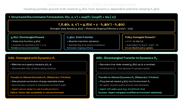
Imitation learning methods like Generative Adversarial Imitation Learning (GAIL) train an agent to mimic expert behavior by matching state-action occupancy measures $\rho(s, a)$ . While GAIL efficiently trains an imitating policy, its learned discriminator $D(s, a)$ is fundamentally entangled with the training environment's transition dynamics $\mathcal{P}_1(s' \mid s, a)$ .

If the environment changes—such as when a robot suffers a jammed motor, moves to a surface with different friction, or encounters newly placed obstacles ( $\mathcal{P}_2$ )—GAIL's discriminator outputs meaningless values. Because GAIL learned how to move rather than what the goal is, the policy fails completely.

To enable true policy transfer across changing physical dynamics, the agent must recover the ground-truth reward function $R^*(s)$ through Inverse Reinforcement Learning (IRL). However, classical Maximum Entropy IRL (Ziebart et al., 2008) requires running an entire forward reinforcement learning loop at every optimization step, making it computationally prohibitive for complex continuous control tasks.

Adversarial Inverse Reinforcement Learning (AIRL) (Fu, Luo, & Levine, 2018) solves both problems simultaneously:

It preserves the sample efficiency of adversarial training (updating the policy with single-step transitions).
It mathematically decomposes the discriminator to disentangle the true state reward $g_\theta(s)$ from transition-dependent potential shaping $h_\phi(s)$ .
The recovered reward function $g_\theta(s)$ is provably invariant to environment dynamics, allowing an agent to re-plan and succeed in radically modified environments.

Think of It Like This

Teaching an agility course to a dog: Motion mimicry vs. Goal understanding

Imagine training an agility dog. A champion handler demonstrates an agility course: sprinting through a tunnel, leaping over a red hurdle, and crossing the finish line where a bowl of food is placed.

The GAIL Approach (Motion Mimicry): The student dog memorizes the exact running speed, leap timing, and paw placements from the demonstration.

As long as the hurdles remain in their exact original spots, the dog performs well. But if you move the red hurdle three meters to the left, the dog leaps into empty air, crashes into the displaced obstacle, and gets disqualified. It mimicked the physical motion without understanding the objective.
The AIRL Approach (Reward Disentanglement): The student dog observes the demonstration and separates the task into two components:
1. Shaping Potential ( $h_\phi$ ): Jumping over hurdles was just the temporary physical maneuvering needed to navigate the specific arena layout.
2. Ground-Truth Reward ( $g_\theta$ ): The true prize is reaching the finish line to eat the food.

When placed in a new arena with rearranged hurdles, the dog does not blindly replay the old paw placements. It plans a new path around the shifted hurdles and sprints straight to the finish line.

Where the analogy stops: A dog has biological senses to smell food and perceive rewards directly. In inverse reinforcement learning, the environment provides zero reward signals to the agent during demonstrations. AIRL must isolate the true reward $g_\theta(s)$ entirely through the mathematical structure of its adversarial discriminator.

How It Actually Works

The Structured Discriminator and Reward Disentanglement

In Maximum Entropy Inverse Reinforcement Learning, the optimal policy takes the energy-based form $\pi^*(a \mid s) \propto \exp(Q^*(s, a) - V^*(s))$ .

AIRL incorporates this formulation directly into a GAN discriminator by structuring $D(s, a, s')$ to contrast a learned advantage function against the generator policy probability $\pi(a \mid s)$ :

D_{\theta, \phi}(s, a, s') = \frac{\exp\big(f_{\theta, \phi}(s, a, s')\big)}{\exp\big(f_{\theta, \phi}(s, a, s')\big) + \pi(a \mid s)}

1. Reward Disentanglement Parameterization

According to policy invariance under reward shaping (Ng, Harada, & Russell, 1999), two reward functions share the same optimal policy if and only if they differ by a potential difference $\gamma \Phi(s') - \Phi(s)$ .

AIRL explicitly parameterizes the advantage function $f_{\theta, \phi}$ to separate the true reward from the shaping potential:

f_{\theta, \phi}(s, a, s') = \underbrace{g_\theta(s)}_{\text{Disentangled True Reward}} + \underbrace{\gamma \cdot h_\phi(s') - h_\phi(s)}_{\text{Potential Shaping Difference}}

$g_\theta(s)$ : A neural network that estimates the ground-truth reward, restricted to depend only on state $s$ .
$h_\phi(s)$ : A neural network that estimates the state potential function, absorbing transition dynamics and value baseline differences.

2. The Theoretical Guarantee (Fu et al., 2018)

When $g_\theta$ is parameterized as a state-only function $g_\theta(s)$ , the discriminator's global optimum satisfies:

g_\theta(s) = R^*(s) + c

where $R^*(s)$ is the true environment reward and $c$ is a constant. The learned reward $g_\theta(s)$ is disentangled from transition dynamics $\mathcal{P}(s' \mid s, a)$ , meaning it can be directly exported to an environment with different physics or obstacle layouts.

3. Adversarial Training Loop

Training alternates between updating the discriminator and the generator policy:

Discriminator Update: Train $(g_\theta, h_\phi)$ using binary cross-entropy on expert transitions vs. policy transitions: $\max_{\theta, \phi} \mathbb{E}_{(s, a, s') \sim \mathcal{D}_E} \big[ \log D_{\theta, \phi}(s, a, s') \big] + \mathbb{E}_{(s, a, s') \sim \pi} \big[ \log \big(1 - D_{\theta, \phi}(s, a, s')\big) \big]$
Policy Update: Train policy $\pi$ via policy gradients (e.g. TRPO or PPO) using the surrogate reward: $\hat{r}(s, a, s') = \log D(s, a, s') - \log\big(1 - D(s, a, s')\big) = f_{\theta, \phi}(s, a, s') - \log \pi(a \mid s)$

Worked numerical example

Let us trace a single transition update under AIRL.

Transition Setup:

Current state $s$ , action $a$ , and next state $s'$ .
Learner policy probability: $\pi(a \mid s) = 0.20$ .
Learned state reward network: $g_\theta(s) = 2.0$ .
Learned potential function evaluations: $h_\phi(s) = 1.0$ , $h_\phi(s') = 1.5$ .
Discount factor: $\gamma = 0.90$ .

Step 1: Compute Shaped Advantage Function $f(s, a, s')$

f_{\theta, \phi}(s, a, s') = g_\theta(s) + \gamma h_\phi(s') - h_\phi(s)

f_{\theta, \phi}(s, a, s') = 2.0 + 0.90(1.5) - 1.0 = 2.0 + 1.35 - 1.0 = 2.35

Step 2: Compute Discriminator Output $D(s, a, s')$

Evaluate the exponential advantage:

\exp(f) = \exp(2.35) \approx 10.4856

Evaluating the structured discriminator:

D(s, a, s') = \frac{\exp(f)}{\exp(f) + \pi(a \mid s)} = \frac{10.4856}{10.4856 + 0.20} = \frac{10.4856}{10.6856} \approx 0.9813

Because $D \approx 0.98$ , the discriminator strongly suspects this transition came from an expert.

Step 3: Compute Policy Surrogate Reward $\hat{r}(s, a, s')$

\hat{r}(s, a, s') = f(s, a, s') - \ln \pi(a \mid s)

\ln(0.20) \approx -1.6094

\hat{r} = 2.35 - (-1.6094) = 2.35 + 1.6094 = 3.9594

Step 4: Dynamics Transfer Demonstration

Suppose the robot transitions to a modified environment $\mathcal{P}_2$ with higher friction, causing action $a$ from state $s$ to transition to state $s''$ instead of $s'$ , where $h_\phi(s'') = 0.80$ .

The shaping term shifts: $0.90(0.80) - 1.0 = 0.72 - 1.0 = -0.28$ .
The advantage shifts: $f = 2.0 - 0.28 = 1.72$ .
Crucially, the recovered reward function $g_\theta(s) = 2.0$ remains identical.

The agent transfers $g_\theta(s)$ directly into environment $\mathcal{P}_2$ and re-optimizes a policy that accommodates the new friction.

Code

1import math2from typing import Dict, Tuple3
4
5class AdversarialInverseRLSimulator:6    """Demonstrates Adversarial Inverse Reinforcement Learning (AIRL; Fu et al., 2018):7
8    1. Structured Discriminator: D = exp(f) / [exp(f) + pi(a | s)]9    2. Advantage Decomposition: f = g_theta(s) + gamma * h_phi(s') - h_phi(s)10    3. Surrogate Reward: r_hat = f - ln pi(a | s)11    4. Reward Transfer across modified transition dynamics12    """13
14    def __init__(self, gamma: float = 0.90) -> None:15        self.gamma = gamma16
17    def compute_shaped_advantage(18        self,19        g_reward: float,20        h_current: float,21        h_next: float,22    ) -> float:23        """Calculates f(s, a, s') = g(s) + gamma * h(s') - h(s)."""24        return round(g_reward + self.gamma * h_next - h_current, 4)25
26    @staticmethod27    def compute_discriminator_output(28        advantage_f: float,29        policy_prob: float,30    ) -> Tuple[float, float]:31        """Calculates D(s, a, s') = exp(f) / [exp(f) + pi(a | s)]."""32        exp_f = math.exp(advantage_f)33        d_val = exp_f / (exp_f + policy_prob)34        return round(exp_f, 4), round(d_val, 4)35
36    @staticmethod37    def compute_surrogate_reward(38        advantage_f: float,39        policy_prob: float,40    ) -> float:41        """Calculates policy update reward: r_hat = f - ln pi(a | s)."""42        log_pi = math.log(policy_prob)43        return round(advantage_f - log_pi, 4)44
45
46# Initialize simulator with worked numerical example parameters47airl = AdversarialInverseRLSimulator(gamma=0.90)48
49# 1. Primary Environment P_1 Evaluation50g_state = 2.0  # Disentangled ground-truth reward g_theta(s)51h_curr = 1.0  # State potential h_phi(s)52h_next_p1 = 1.5  # State potential in environment P_1: h_phi(s')53pi_a_s = 0.20  # Policy probability pi(a | s)54
55f_p1 = airl.compute_shaped_advantage(g_state, h_curr, h_next_p1)56exp_f_p1, d_p1 = airl.compute_discriminator_output(f_p1, pi_a_s)57r_surrogate_p1 = airl.compute_surrogate_reward(f_p1, pi_a_s)58
59print("=== Environment P_1 Evaluation ===")60print(f"Shaped Advantage f(s, a, s'): {f_p1:.2f}")61# -> Shaped Advantage f(s, a, s'): 2.3562print(f"exp(f): {exp_f_p1:.4f}")63# -> exp(f): 10.485664print(f"Discriminator D: {d_p1:.4f}")65# -> Discriminator D: 0.981366print(f"Surrogate Reward r_hat: {r_surrogate_p1:.4f}")67# -> Surrogate Reward r_hat: 3.959468print(f"Disentangled State Reward g_theta(s): {g_state:.2f}")69# -> Disentangled State Reward g_theta(s): 2.0070
71# 2. Transfer to Modified Dynamics P_2 (Altered Friction / Obstacles)72h_next_p2 = 0.80  # Next state potential shifts under new physics: h_phi(s'')73f_p2 = airl.compute_shaped_advantage(g_state, h_curr, h_next_p2)74
75print("\n=== Environment P_2 (Modified Dynamics) Transfer ===")76print(77    f"New Shaped Advantage f(s, a, s''): {f_p2:.2f} (absorbed by potential h)"78)79# -> New Shaped Advantage f(s, a, s''): 1.72 (absorbed by potential h)80print(f"Exported Ground-Truth Reward g_theta(s): {g_state:.2f} (UNCHANGED!)")81# -> Exported Ground-Truth Reward g_theta(s): 2.00 (UNCHANGED!)82
83# Verification assertions84assert f_p1 == 2.3585assert exp_f_p1 == 10.485686assert d_p1 == 0.981387assert r_surrogate_p1 == 3.959488assert g_state == 2.0089assert f_p2 == 1.72

Watch Out For

Action-Dependent Reward Ambiguity and Entanglement

A frequent mistake when extending AIRL is allowing the reward network to condition on actions: $g_\theta(s, a)$ .

While action-dependent rewards seem more expressive, conditioning on action $a$ breaks the uniqueness guarantees of potential-based reward shaping. If $g$ depends on $a$ , the potential difference $\gamma h_\phi(s') - h_\phi(s)$ can no longer uniquely absorb the environment's transition dynamics $\mathcal{P}(s' \mid s, a)$ . The learned reward function becomes mathematically entangled with the specific transition probabilities of the training environment.

When an action-dependent reward $g_\theta(s, a)$ is transferred to an environment with modified dynamics (such as a robotic arm with an altered payload or altered joint damping), the agent learns erratic, divergent policies that exploit the obsolete shaping artifacts.

The Fix: Always restrict $g_\theta$ to be a state-only function $g_\theta(s)$ . Fu et al. (Theorem 5.1) prove that when $g$ is state-only, the learned reward function is guaranteed to recover the true ground-truth reward up to an additive constant, ensuring robust transfer across arbitrary dynamic shifts.

The Quick Version

AIRL recovers transferable ground-truth reward functions $g_\theta(s)$ by structuring the adversarial discriminator: $D = \frac{\exp(f)}{\exp(f) + \pi}$ .
The advantage function decomposes into disentangled state reward and potential shaping: $f(s, a, s') = g_\theta(s) + \gamma h_\phi(s') - h_\phi(s)$ .
Unlike GAIL (which mimics motion trajectories that collapse when physics change), AIRL recovers the underlying goal, enabling seamless transfer to altered dynamics environments.
To guarantee mathematical reward disentanglement and prevent dynamics leakage, $g_\theta$ must be strictly constrained to be a state-only function $g_\theta(s)$ .