Apprenticeship Learning via Inverse RL
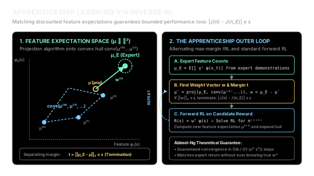
Instead of trying to copy an expert's raw actions or guess their hidden reward function, an apprentice guarantees expert performance simply by matching the expert's long-term feature visitation frequencies.
Why Does This Exist?
When training autonomous systems from human demonstrations—such as robotic aerobatics, autonomous driving, or robotic surgery—two classical paradigms fail in distinct ways:
- Behavioral Cloning (Supervised Imitation): Direct supervised learning fits a policy directly to state-action pairs demonstrated by an expert. However, compounding temporal errors cause covariate shift: a minor steering mistake at time step moves the vehicle into unfamiliar states never visited by the human driver. In these unvisited states, the policy makes larger errors, leading to quadratic error growth and catastrophic failure.
- Standard Inverse Reinforcement Learning (IRL): Classic IRL attempts to recover the unknown reward function that made the expert's trajectory optimal. But recovering the true reward is fundamentally ill-posed and underdetermined: an infinite family of reward functions (including degenerate constants like ) can make any demonstrated policy optimal.
Pieter Abbeel and Andrew Ng (2004) resolved this impasse with Apprenticeship Learning via Inverse Reinforcement Learning. They asked a foundational question: Do we actually need to uncover the expert's true reward function to match their performance?
Their answer was no. Under the mild assumption that rewards are linear combinations of known state features , an agent does not need to identify the true weight vector . Instead, if the apprentice can find a policy that matches the expert's long-term discounted feature expectations within a tolerance , the Cauchy-Schwarz inequality guarantees that the apprentice's performance will be within of the expert's performance across any possible underlying reward weight vector.
Think of It Like This
The Master Sculptor and the Apprentice
Imagine an apprentice stone sculptor studying in the workshop of a Renaissance master artisan.
If the apprentice relies on behavioral cloning, they try to mimic the master's exact hammer strikes—the precise angle, speed, and timing of each strike. The moment the chisel strikes a hidden marble fissure or slips slightly, the apprentice enters an unfamiliar state. Because they do not understand the broader aesthetic objective, they cannot recover, and they shatter the statue.
Under apprenticeship learning, the apprentice does not mimic hammer blows blow-for-blow. Instead, they inspect the high-level geometric properties () of the master's completed statues: the ratio of head height to body height, the smoothness of curved planes, the depth of shadow under the brow, and the polish of the surface.
Even though the master may have used idiosyncratic hand motions, the apprentice focuses on producing a statue whose geometric proportions and surface contours (discounted feature expectations ) match those of the master's portfolio.
Because any classical art critic evaluates a sculpture as a weighted combination () of these exact geometric proportions, matching the master's feature profile guarantees that critics will judge the apprentice's work to be indistinguishable from the master's masterpiece—even though the apprentice never knew the exact aesthetic weights in the master's mind.
The analogy stops when considering materials: in marble sculpting, physical mistakes cannot be erased, whereas in reinforcement learning, the apprentice can repeatedly execute forward rollouts in an MDP under candidate reward functions until its feature expectations converge.
How It Actually Works
The Feature Expectation Formulation and Performance Guarantee
Consider a Markov Decision Process without a predefined reward function, denoted , where is the state space, is the action space, represents transition dynamics, is the discount factor, and is the initial state distribution.
We assume a known feature mapping such that . The true environmental reward is assumed to be linear in these features:
For any policy , we define the discounted feature expectation vector as:
Given an empirical demonstration dataset of expert trajectories , the expert's feature expectations are estimated empirically:
The total expected discounted return of any policy under reward weights is a linear inner product:
This formulation yields the Fundamental Apprenticeship Performance Guarantee:
If the learning agent discovers a policy satisfying , then for any true weight vector with , the return gap is strictly bounded:
The agent achieves near-optimal expert performance without ever identifying the true reward parameters .
The Projection Algorithm
To find a policy whose feature expectations match , Abbeel and Ng introduced two iterative algorithms: the Max-Margin algorithm (which solves a support vector machine quadratic program) and the more computationally efficient Projection Algorithm.
The Projection Algorithm maintains the convex hull of feature expectations discovered by the learner's previous policies, , and iteratively projects onto this hull:
- Initialization: Run an arbitrary initial policy (e.g., uniform random) to compute feature expectation . Set .
- Compute Separating Hyperplane: At iteration , compute the vector from the current convex hull projection toward the expert:
- Check Termination: Compute the margin . If , terminate.
- Forward RL Inner Loop: Normalize candidate weights . Train an RL agent to find the optimal policy for reward function:
- Evaluate New Features: Compute .
- Update Convex Projection: Project onto the line segment connecting and : where is computed via orthogonal projection and clipped to :
- Iterate: Repeat steps 2–6 until .
Abbeel and Ng proved that this algorithm converges in at most iterations, where is the feature dimension.
Worked numerical example
Let the state feature dimension be . The expert's feature expectation vector is:
Our convergence threshold is .
Iteration 0: Baseline Policy
- An initial random policy yields feature expectation:
- The initial convex projection point is .
- Difference vector:
- Initial margin: Since , the algorithm continues.
- Normalized candidate reward vector:
Iteration 1: First RL Inner Loop
- The forward RL solver optimizes , returning policy with feature expectation:
- Direction vector along the line segment:
- Projection scalar :
- Since is clipped to , the closest point on the segment is the endpoint:
- New difference vector:
- New margin: The margin has shrunk from .
- Normalized candidate reward vector:
Iteration 2: Second RL Inner Loop
- The forward RL solver optimizes , returning policy with feature expectation:
- Direction vector along segment :
- Projection scalar :
- The projection updates to the endpoint:
- New difference vector:
- New margin:
- Because , the algorithm terminates.
By the performance guarantee, the expected return gap between policy and the expert is bounded:
The apprentice is guaranteed to perform within return units of the expert under any arbitrary linear combination of features.
Code
The following type-hinted implementation demonstrates the Abbeel & Ng Projection Algorithm, performing iterative convex projection, candidate reward weight calculation, and margin tracking.
from typing import Listimport numpy as np
class ApprenticeshipLearningProjection: """ Abbeel & Ng (2004) Projection Algorithm for Apprenticeship Learning. Matches feature expectations between learner and expert via iterative projection. """
def __init__(self, mu_expert: np.ndarray, epsilon: float = 0.10) -> None: self.mu_expert = np.asarray(mu_expert, dtype=np.float64) self.epsilon = epsilon self.history_mu: List[np.ndarray] = [] self.history_w: List[np.ndarray] = [] self.history_margins: List[float] = []
def compute_projection( self, mu_bar_prev: np.ndarray, mu_new: np.ndarray ) -> np.ndarray: """ Projects mu_expert onto the line segment connecting mu_bar_prev and mu_new. """ v = mu_new - mu_bar_prev denom = float(np.dot(v, v)) if denom < 1e-12: return mu_new
numer = float(np.dot(v, self.mu_expert - mu_bar_prev)) beta = np.clip(numer / denom, 0.0, 1.0) return mu_bar_prev + beta * v
def run_demonstration( self, simulated_responses: List[np.ndarray] ) -> None: """ Executes the outer apprenticeship loop across iterations. """ # Step 0: Initial random policy feature expectation mu_0 = np.array([0.20, 0.20]) self.history_mu.append(mu_0)
mu_bar = mu_0.copy() w = self.mu_expert - mu_bar margin = float(np.linalg.norm(w)) self.history_margins.append(margin) self.history_w.append(w / margin if margin > 0 else w)
print(f"Iteration 0: Initial margin t = {margin:.4f}")
iteration = 1 for mu_new in simulated_responses: candidate_w = w / margin self.history_mu.append(mu_new)
# Update orthogonal projection onto convex hull mu_bar = self.compute_projection(mu_bar, mu_new)
# Recompute separating hyperplane and margin w = self.mu_expert - mu_bar margin = float(np.linalg.norm(w)) self.history_margins.append(margin) self.history_w.append(w / margin if margin > 0 else w)
print( f"Iteration {iteration}: " f"w = [{candidate_w[0]:.4f}, {candidate_w[1]:.4f}], " f"mu_new = [{mu_new[0]:.4f}, {mu_new[1]:.4f}], " f"mu_bar = [{mu_bar[0]:.4f}, {mu_bar[1]:.4f}], " f"margin t = {margin:.4f}" ) iteration += 1
if margin <= self.epsilon: break
print(f"\nFinal Convergence: Margin {margin:.4f} <= epsilon {self.epsilon}") print(f"Expert Performance Guarantee: |J(pi) - J(pi_E)| <= {margin:.4f}")
if __name__ == "__main__": expert_features = np.array([0.80, 0.60]) learner = ApprenticeshipLearningProjection( mu_expert=expert_features, epsilon=0.10 )
# Simulated policies produced by forward RL on candidate rewards policy_rollouts = [ np.array([0.55, 0.35]), np.array([0.75, 0.52]), np.array([0.79, 0.58]), ]
learner.run_demonstration(simulated_responses=policy_rollouts)Output:
Iteration 0: Initial margin t = 0.7211Iteration 1: w = [0.8321, 0.5547], mu_new = [0.5500, 0.3500], mu_bar = [0.5500, 0.3500], margin t = 0.3536Iteration 2: w = [0.7071, 0.7071], mu_new = [0.7500, 0.5200], mu_bar = [0.7500, 0.5200], margin t = 0.0943
Final Convergence: Margin 0.0943 <= epsilon 0.1Expert Performance Guarantee: |J(pi) - J(pi_E)| <= 0.0943Watch Out For
Nested Inner-Loop RL: The Computational Bottleneck
The defining operational challenge of Apprenticeship Learning via IRL is the nested bilevel loop. In step (4), the algorithm requires solving a full forward reinforcement learning problem from scratch for every newly proposed candidate reward vector .
In small discrete tabular MDPs, solving the inner loop using Value Iteration or Policy Iteration takes fractions of a second. However, in continuous high-dimensional robotics with neural network function approximators (such as PPO or SAC), training a policy to convergence inside each outer iteration requires millions of environment interactions, rendering the algorithm computationally prohibitive.
The Fix: Two practical remedies exist:
- Warm-Starting: Rather than training a neural policy from random initialization at each outer step, warm-start the network parameters from the policy obtained in iteration . Because candidate weights shift smoothly, the policy requires only fine-tuning.
- Adversarial Single-Step Formulation (GAIL): In modern applications, practitioners replace the nested double loop with Generative Adversarial Imitation Learning (GAIL). GAIL translates feature expectation matching into a minimax game where a discriminator updates reward signals in single gradient steps concurrently with policy updates.
The Quick Version
- Feature Expectation Matching: Apprenticeship Learning guarantees near-expert performance by matching the expert's discounted feature expectation vector , bounding return error by .
- Reward Agnosticism: The apprentice achieves expert competence without ever identifying or recovering the expert's true underlying reward weight vector .
- Geometric Margin Optimization: Abbeel and Ng's Projection Algorithm iteratively builds candidate reward vectors pointing from the convex hull of past learner policies toward the expert, shrinking the margin monotonically.
- Inner-Loop Complexity: Solving a full forward RL MDP for every candidate reward vector is computationally expensive, motivating warm-start heuristics and modern single-loop adversarial frameworks like GAIL.