Cooperative vs. Competitive Environments
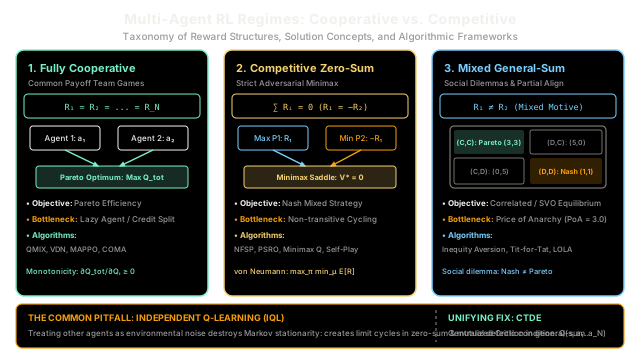
Multi-agent reinforcement learning divides into three distinct game-theoretic regimes based on reward structure: fully cooperative teams, competitive zero-sum adversaries, and mixed-motive social dilemmas. Each regime demands fundamentally different optimization criteria, ranging from Pareto coordination to minimax saddle points and reciprocal contracts.
Why Does This Exist?
In single-agent reinforcement learning, an agent operates inside an environment governed by stationary transition dynamics , optimizing a solitary scalar objective . However, when multiple autonomous agents share an ecosystem—whether autonomous vehicles at an intersection, high-frequency algorithmic traders, warehouse robot swarms, or strategic game-playing bots—the Markov property collapses from the viewpoint of any individual participant.
The environmental next-state distribution depends on the joint action of all agents:
Because other agents update their policies concurrently during training, the effective transition dynamics perceived by Agent fluctuate continuously. An action that yielded high reward at iteration 100 may lead to failure at iteration 200 simply because an opponent adapted its counter-strategy.
Beyond non-stationarity, what constitutes "optimal behavior" changes entirely based on how the reward functions relate to one another:
- Fully Cooperative Teams (): Agents share a single team reward. The objective is collective Pareto optimality, but agents face the Multi-Agent Credit Assignment problem—identifying which specific agent's action contributed to team success versus which agent was a "lazy rider."
- Competitive Zero-Sum Games (): One agent's gain is exactly another's loss. Standard gradient ascent fails because agents oscillate in non-convergent limit cycles (e.g., Rock-Paper-Scissors). Optimal behavior requires finding minimax Nash equilibria where policies are mathematically unexploitable.
- Mixed-Motive General-Sum Games (): Individual and collective interests clash (e.g., Prisoner's Dilemma, traffic congestion). Selfish individual optimization causes agents to collapse into mutually destructive Nash equilibria, creating a severe Price of Anarchy.
Understanding these three distinct interaction regimes is vital: an algorithm engineered for cooperative teams (such as QMIX) will fail completely in competitive or mixed-motive settings, and vice versa.
Think of It Like This
The spectrum of human games: rowing shells, chessboards, and rush-hour highways
Consider how human coordination shifts across three familiar scenarios:
- Rowing an 8-person crew shell (Fully Cooperative): Every rower on the team pulls with the exact same objective: crossing the finish line first. If the boat wins, all 8 rowers receive gold medals; if one rower catches a crab, the entire boat capsizes. The algorithmic challenge is pure synchronization and eliminating "free riders"—ensuring that rowers in the middle do not slack off while letting the stroke and bow oarsmen do all the physical work.
- Tournament Chess (Competitive Zero-Sum): White receives for winning, Black receives , and a draw is . There is zero possibility of mutual benefit. Any tactical advantage granted to your opponent directly destroys your own survival. Optimal play is strictly adversarial minimax: you must assume that your opponent will find the most punishing response to every piece you move, forcing you to play non-exploitable defensive lines.
- Rush-hour highway traffic (Mixed General-Sum): Hundreds of independent commuters share a multi-lane highway. If every driver maintains a steady speed, leaves a 2-second gap, and merges smoothly, traffic flows smoothly for everyone (the Pareto social optimum). However, each individual driver has a selfish incentive to weave aggressively between lanes and tailgate to shave 10 seconds off their personal commute. When every driver adopts this selfish dominant strategy, the highway descends into total gridlock (the Nash equilibrium trap).
Where the analogy stops: human beings navigate these dilemmas using cultural norms, language, legal contracts, and emotional facial expressions (guilt, anger, gratitude). Reinforcement learning agents possess only numerical scalar tensors and observation vectors, requiring rigorous game-theoretic loss functions and factorization architectures to achieve stable coordination.
How It Actually Works
Game-Theoretic Taxonomy and Solution Concepts
Multi-agent reinforcement learning is formalized mathematically as a Markov Game (or Stochastic Game), defined by the tuple , where:
- is the set of agents.
- is the global state space.
- is the action space of agent , forming the joint action space .
- defines transition dynamics conditioned on joint action .
- is the reward function for agent .
The expected discounted return for agent under joint policy is:
The Nash Equilibrium Solution Concept
In multi-agent environments, a single "optimal policy" does not exist in isolation. Instead, outcomes are evaluated using game-theoretic equilibria.
A joint policy is a Nash Equilibrium if no agent can unilaterally increase its expected return by deviating to another policy , holding all other agents' policies fixed:
┌────────────────────────────────────────────────────────┐ │ The Three Multi-Agent Interaction Regimes │ └───────────────────────────┬────────────────────────────┘ ┌─────────────────────────────────┼─────────────────────────────────┐ │ │ │┌────────▼──────────────┐ ┌──────────▼────────────┐ ┌────────────▼──────────┐│ 1. Fully Cooperative │ │ 2. Competitive ZeroSum│ │ 3. Mixed General-Sum ││ R₁ = R₂ = ... = R_N │ │ ∑ Rᵢ = 0 (R₁ = -R₂) │ │ R₁ ≠ R₂ (Mixed Motive)││ Pareto Optimality │ │ Minimax Saddle Point │ │ Social Dilemma Trap ││ VDN, QMIX, MAPPO │ │ Self-Play, NFSP, PSRO │ │ LOLA, Inequity Averse │└───────────────────────┘ └───────────────────────┘ └───────────────────────┘Regime 1: Fully Cooperative Games (Common Payoffs)
In cooperative games, all agents share a single team reward:
1. Solution Concept: Pareto Optimality
Because payoffs are identical, there is no conflict of interest. The goal is achieving Pareto Optimality: a joint policy such that no other policy can increase any agent's return without decreasing another's.
2. The Core Pathology: Multi-Agent Credit Assignment
When the team receives a scalar reward , how does Agent 1 know whether its individual action helped or hurt the outcome? If Agent 1 scores a goal while Agent 2 was caught out of position, both receive identical reward signals. Naive learning leads to the lazy agent problem, where a subset of agents learns to do all the work while others wander aimlessly.
3. Algorithmic Frameworks
- Value Factorization (VDN, QMIX): In Centralized Training with Decentralized Execution (CTDE), a centralized Critic estimates the joint action-value function as a monotonic combination of individual agent utilities : This guarantees the Individual-Global-Max (IGM) condition: decentralized greedy actions automatically maximize global team value .
- Counterfactual Multi-Agent Policy Gradients (COMA): Employs a counterfactual baseline that marginalizes out an agent's individual action while keeping all teammates' actions fixed: This directly measures Agent 's distinct marginal contribution to team success.
Regime 2: Competitive Zero-Sum Games (Adversarial)
In two-player competitive games, rewards sum to zero:
1. Solution Concept: The Minimax Theorem
Under von Neumann's Minimax Theorem (1928), for any two-player zero-sum game, the Nash equilibrium coincides exactly with the minimax strategy:
The value is the unique game-theoretic value of the game. At this saddle point, Player 1 plays a strategy that guarantees expected return at least against any possible opponent strategy, even an adversary with perfect knowledge of Player 1's policy.
2. The Core Pathology: Non-Transitive Cycling
In games with circular dominance (such as Rock-Paper-Scissors or Poker), deterministic pure strategies are completely exploitable. If Player 1 plays pure Rock, Player 2 adapts to Paper; Player 1 then adapts to Scissors; Player 2 adapts to Rock. Naive gradient descent chases this loop endlessly in non-convergent limit cycles. The solution requires learning stochastic mixed strategies .
3. Algorithmic Frameworks
- Self-Play: Training an agent against historical checkpoints of itself (AlphaGo, AlphaZero).
- Fictitious Play and NFSP (Neural Fictitious Self-Play): Agents train against the average historical strategy of their opponent rather than only the latest step, proving mathematical convergence to mixed Nash equilibria.
- Policy Space Response Oracles (PSRO): Frames multi-agent learning as a meta-game, discovering a population of diverse sub-policies via reinforcement learning and computing meta-game Nash distributions via linear programming.
Regime 3: Mixed-Motive General-Sum Games (Social Dilemmas)
In general-sum games, rewards are arbitrary and neither strictly equal nor strictly opposing ( and ).
1. The Core Pathology: The Social Dilemma Trap
General-sum games are characterized by social dilemmas where individual rationality contradicts collective welfare. The defining example is the Prisoner's Dilemma:
- If both cooperate, both earn .
- If one defects while the other cooperates, the defector earns and the cooperator earns .
- If both defect, both earn .
For each individual player, defecting is a strictly dominant strategy ( and ). Consequently, the unique Nash equilibrium is mutual defection . However, mutual cooperation is strictly Pareto superior!
The Price of Anarchy (PoA) quantifies this systemic inefficiency:
In the Prisoner's Dilemma, . Unchecked selfishness destroys of potential social welfare.
2. Algorithmic Frameworks
- Inequity Aversion (Fehr & Schmidt): Augments an agent's objective with penalties for payoff disparity: Penalizing disadvantageous inequity () and advantageous guilt () encourages agents to escape defection traps.
- Learning with Opponent-Learning Awareness (LOLA): Agents optimize their policy while explicitly accounting for how their gradient step will shape the anticipated learning updates of other agents: This induces cooperative equilibria (such as tit-for-tat reciprocity) in repeated general-sum games.
Worked numerical example
To observe how game dynamics shift across regimes, consider two players with binary actions evaluated across three representative matrix games.
Game 1: Cooperative Coordination Game (Common Payoff)
Both players receive identical payoff: .
- Joint action (Cooperate, Cooperate):
- Joint action (Alternative, Alternative):
- Miscoordination or :
Agent 2: Act 0 Agent 2: Act 1Agent 1: Act 0 10.0 0.0Agent 1: Act 1 0.0 6.0- Optimal Team Return:
- Coordination Risk: While is the global Pareto optimum, is also a local Nash equilibrium. If Agent 1 picks but Agent 2 picks , the team receives . Cooperative value factorization (VDN/QMIX) ensures monotonic convergence to .
Game 2: Zero-Sum Matching Pennies (Competitive Minimax)
Player 1 tries to match; Player 2 tries to mismatch. Payoff .
- Actions: , .
P2: Heads (0) P2: Tails (1)P1: Heads (0) (+1, -1) (-1, +1)P1: Tails (1) (-1, +1) (+1, -1)- Pure Strategy Failure:
- If P1 plays , P2 plays .
- If P1 plays , P2 plays .
- No pure Nash equilibrium exists!
- Minimax Mixed Strategy: Let P1 play Heads with probability , and P2 play Heads with probability . Expected payoff for Player 1: To make Player 1 indifferent to Player 2's action, set . To make Player 2 indifferent to Player 1's action, set .
- Equilibrium Game Value: At the minimax equilibrium and , the expected payoff is mathematically zero, and neither player can be exploited.
Game 3: General-Sum Prisoner's Dilemma (Social Dilemma)
Actions: , .
P2: Cooperate (0) P2: Defect (1)P1: Cooperate (0) (3, 3) (0, 5)P1: Defect (1) (5, 0) (1, 1)- Dominant Strategy Verification:
- For Player 1: If P2 plays , Defect gives . If P2 plays , Defect gives . Defect strictly dominates.
- For Player 2: By symmetry, Defect strictly dominates.
- Nash Equilibrium: Unique equilibrium is mutual defection .
- Social Welfare at Nash: .
- Pareto Optimum: Mutual cooperation .
- Social Welfare at Pareto: .
- Price of Anarchy (PoA): Selfish optimization collapses social welfare by a factor of 3.
Code
The following pure Python script implements the MultiAgentRegimeEvaluator class, verifying cooperative Pareto optimality, zero-sum minimax mixed strategies, and general-sum Price of Anarchy metrics with automated assertions.
from typing import Dict, Tupleimport numpy as np
class MultiAgentRegimeEvaluator: """Evaluates game-theoretic metrics across Cooperative, Zero-Sum, and General-Sum regimes."""
def evaluate_cooperative_game( self, payoff_matrix: np.ndarray, ) -> Tuple[Tuple[int, int], float]: """Finds joint action maximizing common team return in cooperative game.""" best_idx = np.unravel_index(np.argmax(payoff_matrix), payoff_matrix.shape) max_payoff = float(payoff_matrix[best_idx]) return (int(best_idx[0]), int(best_idx[1])), max_payoff
def evaluate_matching_pennies( self, payoff_matrix_p1: np.ndarray, p1_prob_heads: float = 0.5, p2_prob_heads: float = 0.5, ) -> Tuple[float, float]: """Evaluates expected payoff in zero-sum game under mixed strategies.""" # Policy vectors: pi_1 (row player), pi_2 (column player) pi_1 = np.array([p1_prob_heads, 1.0 - p1_prob_heads], dtype=np.float64) pi_2 = np.array([p2_prob_heads, 1.0 - p2_prob_heads], dtype=np.float64)
# Expected return: E[R1] = pi_1 @ R1 @ pi_2 expected_v1 = float(pi_1 @ payoff_matrix_p1 @ pi_2) expected_v2 = -expected_v1 return expected_v1, expected_v2
def evaluate_prisoners_dilemma( self, r1_matrix: np.ndarray, r2_matrix: np.ndarray, ) -> Dict[str, float]: """Calculates Pareto vs Nash payoffs and Price of Anarchy in Prisoner's Dilemma.""" # Action 0 = Cooperate, Action 1 = Defect pareto_welfare = float(r1_matrix[0, 0] + r2_matrix[0, 0]) # (C, C) = 3 + 3 = 6.0 nash_welfare = float(r1_matrix[1, 1] + r2_matrix[1, 1]) # (D, D) = 1 + 1 = 2.0 price_of_anarchy = pareto_welfare / nash_welfare
return { "pareto_welfare": pareto_welfare, "nash_welfare": nash_welfare, "price_of_anarchy": price_of_anarchy, "nash_p1_payoff": float(r1_matrix[1, 1]), "nash_p2_payoff": float(r2_matrix[1, 1]), "pareto_p1_payoff": float(r1_matrix[0, 0]), "pareto_p2_payoff": float(r2_matrix[0, 0]), }
# --- Verification Matching Worked Examples ---evaluator = MultiAgentRegimeEvaluator()
# 1. Cooperative Coordination Game: (C,C)->10.0, (D,D)->6.0, miscoord->0.0coop_matrix = np.array([ [10.0, 0.0], [0.0, 6.0]], dtype=np.float64)
best_joint, best_val = evaluator.evaluate_cooperative_game(coop_matrix)print(f"Cooperative Optimal Action: {best_joint} with Payoff: {best_val:.1f}")# -> Cooperative Optimal Action: (0, 0) with Payoff: 10.0
# 2. Zero-Sum Matching Pennies: P1 matches (+1), P2 mismatches (+1)pennies_p1 = np.array([ [1.0, -1.0], [-1.0, 1.0]], dtype=np.float64)
v1, v2 = evaluator.evaluate_matching_pennies(pennies_p1, p1_prob_heads=0.5, p2_prob_heads=0.5)print(f"Zero-Sum Nash Payoffs: V1={v1:.2f}, V2={v2:.2f}")# -> Zero-Sum Nash Payoffs: V1=0.00, V2=0.00
# 3. General-Sum Prisoner's Dilemmar1_pd = np.array([ [3.0, 0.0], [5.0, 1.0]], dtype=np.float64)
r2_pd = np.array([ [3.0, 5.0], [0.0, 1.0]], dtype=np.float64)
pd_results = evaluator.evaluate_prisoners_dilemma(r1_pd, r2_pd)print(f"Prisoner's Dilemma Price of Anarchy: {pd_results['price_of_anarchy']:.1f}")# -> Prisoner's Dilemma Price of Anarchy: 3.0
print(f"Nash Payoff: ({pd_results['nash_p1_payoff']:.1f}, {pd_results['nash_p2_payoff']:.1f})")# -> Nash Payoff: (1.0, 1.0)
print(f"Pareto Payoff: ({pd_results['pareto_p1_payoff']:.1f}, {pd_results['pareto_p2_payoff']:.1f})")# -> Pareto Payoff: (3.0, 3.0)
# Assertions verifying game-theoretic invariantsassert best_val == 10.0, "Cooperative optimum must equal 10.0"assert v1 == 0.0 and v2 == 0.0, "Zero-sum mixed Nash value must equal 0.0"assert pd_results["price_of_anarchy"] == 3.0, "Price of Anarchy must equal 3.0"print("All multi-agent regime assertions verified successfully.")# -> All multi-agent regime assertions verified successfully.Watch Out For
The Independent Learner Fallacy: Non-Stationarity Limit Cycles
The most common trap in multi-agent reinforcement learning is applying single-agent algorithms—such as independent DQN or independent PPO—by treating all other agents as stationary environmental noise (Independent Q-Learning / IQL).
The Failure Mode:
- In competitive zero-sum games (such as Matching Pennies or Rock-Paper-Scissors), independent Q-learners chase each other's policies indefinitely. Because the transition distribution continuously shifts as the opponent learns, Q-values fail to converge, and policy weights oscillate in chaotic limit cycles rather than stabilizing at the mixed Nash equilibrium.
- In general-sum games (such as Prisoner's Dilemma), independent learners greedily update against the current observed state distribution, inevitably collapsing into the mutual defection trap ().
- In cooperative games, independent learners suffer from the lazy agent syndrome and miscoordination, frequently getting trapped in sub-optimal local equilibria.
The Fix:
- In Cooperative Settings: Use Centralized Training with Decentralized Execution (CTDE) with monotonic value factorization (QMIX) or counterfactual credit assignment (COMA). The Critic conditions on the full joint state and all actions during training, ensuring stationarity.
- In Competitive Settings: Use Self-Play combined with historical policy sampling (Neural Fictitious Self-Play or Policy Space Response Oracles / PSRO). Training against a diverse mixture of past opponent checkpoints prevents limit cycles and forces convergence to robust mixed minimax strategies.
- In Mixed-Motive Settings: Incorporate Opponent-Learning Awareness (LOLA) or Inequity Aversion reward bonuses, enabling agents to shape reciprocal cooperative behaviors and escape social dilemma traps.
The Quick Version
- Fully Cooperative MARL () maximizes common team return; requires value factorization (VDN, QMIX) or counterfactual baselines (COMA) to solve the multi-agent credit assignment and lazy agent problems.
- Competitive Zero-Sum MARL () is governed by von Neumann's Minimax Theorem; optimal strategies are stochastic mixed Nash equilibria learned via self-play, fictitious play (NFSP), or PSRO to prevent limit cycle oscillations.
- Mixed-Motive General-Sum Games () exhibit social dilemmas where selfish dominant strategies lead to Pareto sub-optimal Nash equilibria (Price of Anarchy ); requires reciprocity mechanisms (LOLA) or inequity aversion.
- Never Treat Other Agents as Static Noise: Independent Q-learning destroys Markov stationarity; use CTDE in cooperative teams, self-play distributions in adversarial games, and opponent-shaping in mixed dilemmas.