Markov Games

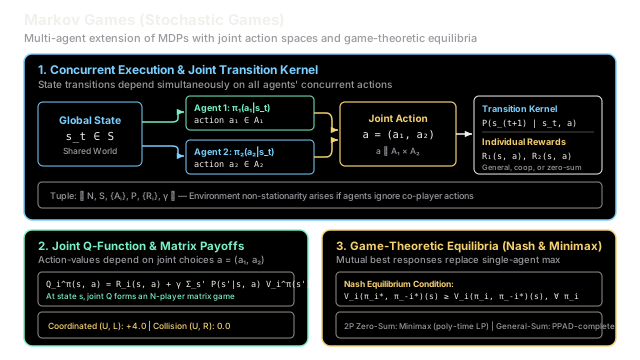
Markov games extend MDPs to multi-agent settings, where state transitions and rewards depend simultaneously on the concurrent actions of all participants.

Why Does This Exist?

In classical single-agent reinforcement learning, the environment is formalized as a Markov Decision Process (MDP). An MDP guarantees environmental stationarity: the transition probability $P(s' | s, a)$ and reward $R(s, a)$ depend solely on the current state $s$ and the lone agent's action $a$ . Under this assumption, the Bellman optimality equation ensures that a stationary optimal policy $\pi^*$ always exists and can be discovered by greedy value iteration: $V^*(s) = \max_a Q^*(s, a)$ .

However, as soon as two or more learning agents operate within the same shared environment—such as autonomous vehicles navigating an intersection, robotic swarms coordinating warehouse logistics, or competing financial algorithms—the single-agent MDP foundation shatters:

Non-Stationarity: From the perspective of any individual agent $i$ , the environment appears non-stationary. As co-players and opponents continuously update their respective policies $\pi_{-i}$ , the observed transition dynamics $P(s' | s, a_i) = \sum_{\mathbf{a}_{-i}} P(s' | s, a_i, \mathbf{a}_{-i}) \boldsymbol{\pi}_{-i}(\mathbf{a}_{-i} | s)$ shift underfoot. An action that led to high rewards yesterday results in catastrophic failure today because other agents altered their behaviors.
Breakdown of the Greedy Max Operator: An agent cannot unilaterally choose to "maximize" its return. The outcome of any action depends entirely on what concurrent choices other agents make at the exact same timestep.
Strategic Interdependence: Agents may cooperate (sharing rewards), compete (zero-sum payoffs), or engage in general-sum mixed-motive interactions requiring mutual coordination or negotiated compromise.

Markov games (first formulated as stochastic games by mathematician Lloyd Shapley in 1953, and introduced to reinforcement learning by Michael Littman in 1994) resolve these challenges. By integrating dynamic programming with game theory, Markov games provide the rigorous mathematical framework for Multi-Agent RL. They replace unilateral maximization with game-theoretic solution concepts—such as the Nash equilibrium and Minimax value—enabling agents to learn stable, mutual best-response strategies.

Think of It Like This

Upgrading from a Solo Simulator to a Multiplayer Traffic Grid

Picture practicing your driving skills in a solo closed-track simulator.

In the solo simulator (single-agent MDP), you are the only car on the track. The physics engine is static and passive. If you turn the steering wheel 30 degrees to the right at 40 mph, your car deterministically glides into the right lane. You can run hundreds of trials, find the exact optimal braking point before each corner, and lock in a single deterministic line. The track will never swerve into you or react to your maneuvers.

Now, imagine taking that exact vehicle onto a busy, un-signaled four-way city intersection occupied by three other human drivers (a Markov game).

You approach the intersection at the same moment as the cross-traffic vehicle. You cannot predict your car's next physical state simply by looking at your own accelerator pedal. If you step on the gas while the cross-traffic driver also steps on the gas, the next state is a high-speed T-bone collision. If both of you slam on the brakes out of extreme caution, you idle indefinitely. If you advance while the other yields, you both safely proceed.

Your steering angle alone no longer dictates reality. The state of the intersection evolves according to the joint vector of all four drivers' pedals and wheels. To avoid gridlock or death, you cannot treat the other cars as inert roadside rocks; you must model their intentions and converge toward shared behavioral conventions (game-theoretic equilibria).

Where the analogy stops: Human drivers rely on eye contact, horn taps, and social traffic conventions. In a formal Markov game, agents execute mathematical policies $\pi_i(a_i | s)$ , and equilibria are computed through matrix-payoff game solvers (such as linear programs or support enumeration) over discounted value functions.

How It Actually Works

Formal Mathematical Definition and Joint Spaces

A Markov game (stochastic game) is formally defined as a tuple:

\langle N, \mathcal{S}, \{\mathcal{A}_i\}_{i=1}^N, P, \{\mathcal{R}_i\}_{i=1}^N, \gamma \rangle

where:

$N$ : The number of participating agents, indexed by $i \in \{1, \dots, N\}$ .
$\mathcal{S}$ : The shared environmental state space.
$\{\mathcal{A}_i\}_{i=1}^N$ : The individual action space for each agent $i$ . The Cartesian product defines the joint action space: $\mathcal{A} = \mathcal{A}_1 \times \mathcal{A}_2 \times \dots \times \mathcal{A}_N$ A joint action vector at timestep $t$ is denoted $\mathbf{a}_t = (a_{1, t}, a_{2, t}, \dots, a_{N, t}) \in \mathcal{A}$ .
$P: \mathcal{S} \times \mathcal{A} \to \Delta(\mathcal{S})$ : The joint transition probability function. The probability of transitioning to state $s'$ depends on the previous state $s$ and the full joint action $\mathbf{a}$ : $P(s' | s, \mathbf{a}) = \Pr(s_{t+1} = s' \mid s_t = s, \mathbf{a}_t = \mathbf{a})$
$\mathcal{R}_i: \mathcal{S} \times \mathcal{A} \times \mathcal{S} \to \mathbb{R}$ : The individual reward function for agent $i$ . Notice that agent $i$ 's reward is determined not just by its own action $a_i$ , but by the concurrent joint action $\mathbf{a}$ of all agents.
$\gamma \in [0, 1)$ : The temporal discount factor for future rewards.

Joint Value Functions and Nash Equilibria

Each agent $i$ chooses actions according to a stochastic policy $\pi_i(a_i | s)$ . Under decentralized execution, the joint policy is the product of individual policies:

\boldsymbol{\pi}(\mathbf{a} | s) = \prod_{i=1}^N \pi_i(a_i | s)

The state-value function for agent $i$ under joint policy $\boldsymbol{\pi}$ is the expected discounted cumulative return:

V_i^{\boldsymbol{\pi}}(s) = \mathbb{E}_{\boldsymbol{\pi}} \left[ \sum_{t=0}^\infty \gamma^t \mathcal{R}_i(s_t, \mathbf{a}_t) \,\Bigg|\, s_0 = s \right]

The joint action-value function satisfies the multi-agent Bellman equation:

Q_i^{\boldsymbol{\pi}}(s, \mathbf{a}) = \mathcal{R}_i(s, \mathbf{a}) + \gamma \sum_{s' \in \mathcal{S}} P(s' | s, \mathbf{a}) V_i^{\boldsymbol{\pi}}(s')

Because all agents' rewards and transitions are coupled, optimal policies cannot be defined unilaterally. Instead, multi-agent reinforcement learning seeks a Markov Perfect Nash Equilibrium.

A joint policy $\boldsymbol{\pi}^* = (\pi_1^*, \dots, \pi_N^*)$ is a Nash equilibrium if for every agent $i \in \{1, \dots, N\}$ and every state $s \in \mathcal{S}$ :

V_i^{(\pi_i^*, \boldsymbol{\pi}_{-i}^*)}(s) \ge V_i^{(\pi_i, \boldsymbol{\pi}_{-i}^*)}(s), \quad \forall \pi_i \in \Pi_i

where $\boldsymbol{\pi}_{-i}^*$ denotes the joint strategy of all agents other than agent $i$ . At equilibrium, no agent can unilaterally increase its expected return by deviating to another policy, assuming all other agents hold their strategies fixed.

Game Classes: Zero-Sum vs. General-Sum

The structure and computational tractability of a Markov game depend heavily on the alignment of reward functions:

Two-Player Zero-Sum Games ( $\mathcal{R}_1 = -\mathcal{R}_2$ ):
- Total conflict: Agent 1's gain is strictly Agent 2's loss.
- Von Neumann's Minimax Theorem guarantees that every state possesses a unique minimax value: $V^*(s) = \max_{\pi_1} \min_{\pi_2} \sum_{a_1, a_2} \pi_1(a_1|s) \pi_2(a_2|s) Q_1^*(s, a_1, a_2)$
- Solvable in polynomial time via linear programming at each Bellman update (e.g., Littman's Minimax-Q algorithm).
Fully Cooperative Games ( $\mathcal{R}_1 = \mathcal{R}_2 = \dots = \mathcal{R}_N$ ):
- Agents share a single identical team reward.
- Reduces to a Multi-Agent MDP (M-MDP) or Dec-POMDP, where agents coordinate on Pareto-optimal joint actions without strategic adversarial counter-play.
General-Sum Games (Arbitrary Rewards):
- Agents have distinct, non-zero-sum preferences (e.g., traffic merging or negotiations).
- Multiple disparate Nash equilibria often coexist (the equilibrium selection problem).
- Computing a Nash equilibrium in general-sum games is PPAD-complete (Polynomial Parity Arguments on Directed graphs), explaining why scalable deep MARL algorithms rely on function approximation and decentralized execution frameworks (like MADDPG, MAPPO, or QMIX).

Worked numerical example

Let us trace a concrete 2-player stochastic game on a 2-state grid:

State Space:
- State $s_0$ : Start state (non-terminal).
- State $s_{\text{goal}}$ : Terminal goal state ( $V_1(s_{\text{goal}}) = V_2(s_{\text{goal}}) = 0.0$ ).
Action Spaces:
- Agent 1: $\mathcal{A}_1 = \{U, D\}$ (Up, Down).
- Agent 2: $\mathcal{A}_2 = \{L, R\}$ (Left, Right).
Transitions and Immediate Payoffs:
- $(U, L)$ (Coordinated Exit): Transitions to $s_{\text{goal}}$ with probability $1.0$ . Payoffs: $\mathcal{R}_1 = +4.0$ , $\mathcal{R}_2 = +4.0$ .
- $(U, R)$ (Collision): State remains $s_0$ with probability $1.0$ . Payoffs: $\mathcal{R}_1 = 0.0$ , $\mathcal{R}_2 = 0.0$ .
- $(D, L)$ (Collision): State remains $s_0$ with probability $1.0$ . Payoffs: $\mathcal{R}_1 = 0.0$ , $\mathcal{R}_2 = 0.0$ .
- $(D, R)$ (Safe Alternate Route): Transitions to $s_{\text{goal}}$ with probability $1.0$ . Payoffs: $\mathcal{R}_1 = +2.0$ , $\mathcal{R}_2 = +2.0$ .
Discount Factor: $\gamma = 0.90$ .
Current Value Estimates: Suppose current estimates are $V_1(s_0) = 2.00$ and $V_2(s_0) = 2.00$ .

Step 1: Compute Joint Action-Values $Q_1(s_0, \mathbf{a})$

Using the multi-agent Bellman equation:

Q_1(s_0, (U, L)) = \mathcal{R}_1(s_0, (U, L)) + \gamma V_1(s_{\text{goal}}) = 4.0 + 0.90 \times 0.0 = 4.00

Q_1(s_0, (U, R)) = \mathcal{R}_1(s_0, (U, R)) + \gamma V_1(s_0) = 0.0 + 0.90 \times 2.00 = 1.80

Q_1(s_0, (D, L)) = \mathcal{R}_1(s_0, (D, L)) + \gamma V_1(s_0) = 0.0 + 0.90 \times 2.00 = 1.80

Q_1(s_0, (D, R)) = \mathcal{R}_1(s_0, (D, R)) + \gamma V_1(s_{\text{goal}}) = 2.0 + 0.90 \times 0.0 = 2.00

By symmetry, $Q_2(s_0, \mathbf{a}) = Q_1(s_0, \mathbf{a})$ for all joint actions.

Step 2: Form the Matrix Payoff Game at State $s_0$

At state $s_0$ , the Q-values form the following symmetric $2 \times 2$ bimatrix game $(Q_1, Q_2)$ :

Agent 1 \ Agent 2	$L$ (Left)	$R$ (Right)
$U$ (Up)	$(4.00, 4.00)$	$(1.80, 1.80)$
$D$ (Down)	$(1.80, 1.80)$	$(2.00, 2.00)$

Step 3: Evaluate Nash Equilibria

Pure Strategy Nash Equilibria:
- Pair $(U, L)$ : If Agent 2 plays $L$ , Agent 1's best response is $U$ ( $4.00 > 1.80$ ). If Agent 1 plays $U$ , Agent 2's best response is $L$ ( $4.00 > 1.80$ ). This is a pure Nash equilibrium with payoff $(4.00, 4.00)$ (Pareto-dominant).
- Pair $(D, R)$ : If Agent 2 plays $R$ , Agent 1's best response is $D$ ( $2.00 > 1.80$ ). If Agent 1 plays $D$ , Agent 2's best response is $R$ ( $2.00 > 1.80$ ). This is also a pure Nash equilibrium with payoff $(2.00, 2.00)$ (risk-dominant).
Mixed Strategy Nash Equilibrium: Let Agent 1 play $U$ with probability $p$ and $D$ with probability $1-p$ .
Let Agent 2 play $L$ with probability $q$ and $R$ with probability $1-q$ .

For Agent 2 to randomize between $L$ and $R$ , the expected payoffs must be equal:
$\mathbb{E}[Q_2 \mid L] = 4.00 p + 1.80 (1 - p) = 1.80 + 2.20 p$ $\mathbb{E}[Q_2 \mid R] = 1.80 p + 2.00 (1 - p) = 2.00 - 0.20 p$
Equating them:
$1.80 + 2.20 p = 2.00 - 0.20 p \implies 2.40 p = 0.20 \implies p = \frac{0.20}{2.40} = \frac{1}{12} \approx 0.0833$
By symmetry:
$q = \frac{1}{12} \approx 0.0833$
Under this mixed equilibrium, both agents achieve an expected return of:
$V_1^{\text{mixed}}(s_0) = 1.80 + 2.20 \left(\frac{1}{12}\right) = 1.80 + 0.1833 = 1.9833$

If both agents coordinate on the Pareto-dominant pure equilibrium $(U, L)$ , the updated state value for state $s_0$ improves from $2.00$ to $V_1(s_0) = 4.00$ .

Code

1import numpy as np2
3
4class MarkovGameSimulator:5    """Simulates a 2-player stochastic Markov game with joint action transitions,6
7    payoff matrices, and Nash equilibrium evaluation.8    """9
10    def __init__(self, gamma: float = 0.90) -> None:11        self.gamma = gamma12        self.actions_p1 = ["U", "D"]13        self.actions_p2 = ["L", "R"]14
15    def compute_joint_q_values(16        self, v_s0: float, v_goal: float = 0.017    ) -> tuple[np.ndarray, np.ndarray]:18        """Computes Q-matrices for Agent 1 and Agent 2 at non-terminal state s_0.19
20        Joint Actions:21        (U, L): Coordinated exit -> R=(+4.0, +4.0), s' = s_goal22        (U, R): Collision       -> R=( 0.0,  0.0), s' = s_023        (D, L): Collision       -> R=( 0.0,  0.0), s' = s_024        (D, R): Suboptimal exit -> R=(+2.0, +2.0), s' = s_goal25        """26        q1 = np.zeros((2, 2), dtype=np.float64)27        q2 = np.zeros((2, 2), dtype=np.float64)28
29        # Joint action (U, L) -> Index (0, 0)30        q1[0, 0] = 4.0 + self.gamma * v_goal31        q2[0, 0] = 4.0 + self.gamma * v_goal32
33        # Joint action (U, R) -> Index (0, 1)34        q1[0, 1] = 0.0 + self.gamma * v_s035        q2[0, 1] = 0.0 + self.gamma * v_s036
37        # Joint action (D, L) -> Index (1, 0)38        q1[1, 0] = 0.0 + self.gamma * v_s039        q2[1, 0] = 0.0 + self.gamma * v_s040
41        # Joint action (D, R) -> Index (1, 1)42        q1[1, 1] = 2.0 + self.gamma * v_goal43        q2[1, 1] = 2.0 + self.gamma * v_goal44
45        return q1, q246
47    def find_pure_nash_equilibria(48        self, q1: np.ndarray, q2: np.ndarray49    ) -> list[tuple[str, str, float, float]]:50        """Identifies all pure strategy Nash equilibria in the 2x2 matrix game."""51        pure_equilibria: list[tuple[str, str, float, float]] = []52
53        for i, a1 in enumerate(self.actions_p1):54            for j, a2 in enumerate(self.actions_p2):55                # Check if a1 is best response to a2: q1[i, j] >= q1[k, j] for all k56                is_br_p1 = bool(np.all(q1[i, j] >= q1[:, j]))57                # Check if a2 is best response to a1: q2[i, j] >= q2[i, k] for all k58                is_br_p2 = bool(np.all(q2[i, j] >= q2[i, :]))59
60                if is_br_p1 and is_br_p2:61                    pure_equilibria.append(62                        (a1, a2, float(q1[i, j]), float(q2[i, j]))63                    )64
65        return pure_equilibria66
67    def compute_mixed_nash_equilibrium(68        self, q1: np.ndarray, q2: np.ndarray69    ) -> tuple[float, float, float, float]:70        """Computes mixed strategy Nash equilibrium (p for U, q for L) and expected payoffs."""71        # Condition for Agent 2: E[Q2|L] == E[Q2|R]72        denom_p = (q2[0, 0] - q2[1, 0]) - (q2[0, 1] - q2[1, 1])73        p = float((q2[1, 1] - q2[1, 0]) / denom_p)74
75        # Condition for Agent 1: E[Q1|U] == E[Q1|D]76        denom_q = (q1[0, 0] - q1[0, 1]) - (q1[1, 0] - q1[1, 1])77        q = float((q1[1, 1] - q1[0, 1]) / denom_q)78
79        # Expected equilibrium returns80        v1_mixed = float(81            p * q * q1[0, 0]82            + p * (1 - q) * q1[0, 1]83            + (1 - p) * q * q1[1, 0]84            + (1 - p) * (1 - q) * q1[1, 1]85        )86        v2_mixed = float(87            p * q * q2[0, 0]88            + p * (1 - q) * q2[0, 1]89            + (1 - p) * q * q2[1, 0]90            + (1 - p) * (1 - q) * q2[1, 1]91        )92
93        return p, q, v1_mixed, v2_mixed94
95
96if __name__ == "__main__":97    np.set_printoptions(precision=4, suppress=True)98
99    sim = MarkovGameSimulator(gamma=0.90)100
101    # Initial state values from the worked numerical example102    v_s0_initial = 2.00103    v_goal = 0.00104
105    # Step 1: Compute joint Q-values106    q1, q2 = sim.compute_joint_q_values(v_s0=v_s0_initial, v_goal=v_goal)107
108    # Step 2: Solve for pure strategy Nash equilibria109    pure_eqs = sim.find_pure_nash_equilibria(q1, q2)110
111    # Step 3: Solve for mixed strategy Nash equilibrium112    p_mix, q_mix, v1_mix, v2_mix = sim.compute_mixed_nash_equilibrium(q1, q2)113
114    print(f"Q1(s_0, (U, L)): {q1[0, 0]:.2f}")115    # -> Q1(s_0, (U, L)): 4.00116
117    print(f"Q1(s_0, (U, R)): {q1[0, 1]:.2f}")118    # -> Q1(s_0, (U, R)): 1.80119
120    print(f"Q1(s_0, (D, L)): {q1[1, 0]:.2f}")121    # -> Q1(s_0, (D, L)): 1.80122
123    print(f"Q1(s_0, (D, R)): {q1[1, 1]:.2f}")124    # -> Q1(s_0, (D, R)): 2.00125
126    print(f"Pure Nash Equilibria count: {len(pure_eqs)}")127    # -> Pure Nash Equilibria count: 2128
129    print(130        f"Pareto-Dominant Equilibrium: ({pure_eqs[0][0]}, {pure_eqs[0][1]}) with payoffs ({pure_eqs[0][2]:.2f}, {pure_eqs[0][3]:.2f})"131    )132    # -> Pareto-Dominant Equilibrium: (U, L) with payoffs (4.00, 4.00)133
134    print(135        f"Risk-Dominant Equilibrium: ({pure_eqs[1][0]}, {pure_eqs[1][1]}) with payoffs ({pure_eqs[1][2]:.2f}, {pure_eqs[1][3]:.2f})"136    )137    # -> Risk-Dominant Equilibrium: (D, R) with payoffs (2.00, 2.00)138
139    print(140        f"Mixed Nash Equilibrium: p(U)={p_mix:.4f}, q(L)={q_mix:.4f}, V1={v1_mix:.4f}"141    )142    # -> Mixed Nash Equilibrium: p(U)=0.0833, q(L)=0.0833, V1=1.9833143
144    # Assert correctness against worked example145    assert np.isclose(q1[0, 0], 4.00, atol=1e-2)146    assert np.isclose(q1[0, 1], 1.80, atol=1e-2)147    assert np.isclose(q1[1, 0], 1.80, atol=1e-2)148    assert np.isclose(q1[1, 1], 2.00, atol=1e-2)149    assert len(pure_eqs) == 2150    assert pure_eqs[0][:2] == ("U", "L")151    assert pure_eqs[1][:2] == ("D", "R")152    assert np.isclose(p_mix, 1 / 12, atol=1e-3)153    assert np.isclose(q_mix, 1 / 12, atol=1e-3)154    assert np.isclose(v1_mix, 1.9833, atol=1e-3)

Watch Out For

Assuming Environment Stationarity by Factoring Transition Dynamics Independently

The most frequent architectural trap in multi-agent reinforcement learning is applying independent single-agent algorithms (like Independent Q-Learning, IQL) directly to a multi-agent environment by treating other agents as static background noise.

Practitioners assume that agent $i$ can learn using a local transition model $P(s' | s, a_i)$ and a scalar Q-function $Q_i(s, a_i)$ . In reality:

The true transition probability $P(s' | s, a_i, \mathbf{a}_{-i})$ is strictly coupled to the actions $\mathbf{a}_{-i}$ of all other agents.
As co-players learn and adapt their policies $\boldsymbol{\pi}_{-i}$ , the marginal transition distribution shifts continuously: $P^{(t)}(s' | s, a_i) = \sum_{\mathbf{a}_{-i}} P(s' | s, a_i, \mathbf{a}_{-i}) \boldsymbol{\pi}_{-i}^{(t)}(\mathbf{a}_{-i} | s)$
Because $P^{(t)}$ changes at every training epoch $t$ , the Markov property is completely violated from the perspective of agent $i$ . Experience collected in earlier replay batches no longer reflects the true underlying transition dynamics, causing severe policy oscillations, policy chasing, and failure to converge.

The Fix: Model the multi-agent nature explicitly:

Centralized Training with Decentralized Execution (CTDE): Use architectures like MADDPG, MAPPO, or QMIX. During training, the critic network evaluates joint action-values $Q(s, a_1, \dots, a_N)$ using global information, while decentralized actor networks execute individual policies $\pi_i(a_i | o_i)$ using local observations during deployment.
Opponent Modeling: Explicitly model the predicted policy distribution of other agents $\hat{\boldsymbol{\pi}}_{-i}(\mathbf{a}_{-i} | s)$ to marginalize transitions accurately.
Equilibrium-Based Value Backups: When operating in small discrete games, employ Minimax-Q or Nash-Q learning to backup values based on game-theoretic equilibria rather than myopic single-agent greedy max operators.

The Quick Version

Multi-Agent Generalization of MDPs: Markov games formalize environments with $N$ concurrent decision-makers, where state transitions $P(s' | s, \mathbf{a})$ and individual rewards $\mathcal{R}_i(s, \mathbf{a})$ depend on the full joint action vector $\mathbf{a} = (a_1, \dots, a_N)$ .
Inherent Non-Stationarity: Treating co-players as part of the environment violates the Markov property because changing policies continuously alter perceived transition dynamics.
Nash Equilibrium Replaces Max: Unilateral maximization ( $\max_a$ ) is invalid; agents instead seek Markov Perfect Nash Equilibria where no agent can unilaterally improve their return by altering their strategy.
Game Classes Dictate Complexity: Two-player zero-sum games possess unique minimax values solvable via linear programming, while general-sum games admit multiple equilibria whose computation is PPAD-complete.