Independent Q-Learning (IQL in MARL)

Each agent learns its own action-values independently, treating teammates as dynamic environment noise rather than intentional decision-makers.

Independent Q-Learning decentralized architecture highlighting the moving target non-stationarity problem and relative overgeneralization dynamics.

Why Does This Exist?

When scaling reinforcement learning to multi-agent systems, centralized learning approaches encounter an immediate exponential bottleneck. In a system with $N$ agents where each agent has $|A|$ discrete actions, the joint action space grows combinatorially:

|\mathbf{\mathcal{A}}| = |A_1| \times |A_2| \times \dots \times |A_N| = |A|^N

Centralized controllers struggle with this dimensional explosion, and in real-world distributed settings (such as autonomous drone swarms or robotic warehouse fleets), low-latency peer-to-peer communication during execution is often impossible.

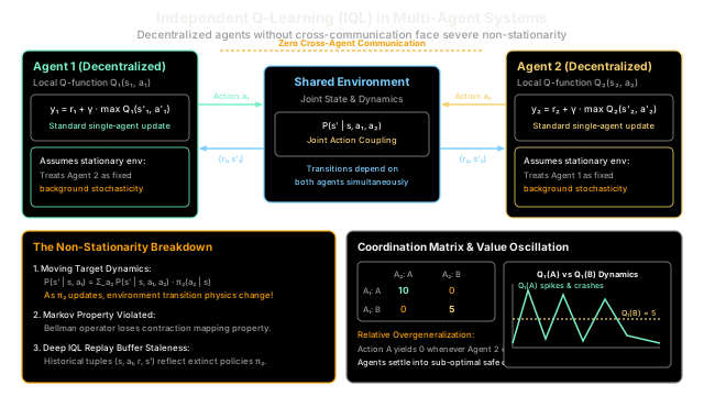
Independent Q-Learning (IQL) (Tan, 1993) provides the most straightforward, scalable decentralized baseline: each agent independently runs standard single-agent Q-learning, choosing its local action $a_i$ based solely on its local observation $s_i$ and reward $r_i$ . Each agent completely ignores the existence of other agents, treating their actions as unobserved environmental stochasticity.

While simple and scalable, IQL introduces a fundamental theoretical flaw: the non-stationarity problem. Because all agents update their policies simultaneously, the environment's transition probabilities and reward landscapes shift continuously beneath each agent's feet, violating the Markov property.

Think of It Like This

Musicians in soundproof isolation booths playing a jazz duet

Imagine a pianist and a drummer attempting to rehearse a complex jazz duet, but they are locked inside separate, completely soundproof isolation booths with no windows and no shared metronome.

Centralized Orchestration: A conductor sits in a control tower with microphones wired to both booths, dictating exact synchronizations. This works well for two musicians, but as an orchestra grows to a hundred players, coordinating every individual finger movement from a single control desk becomes an impossible bottleneck.
The Independent Q-Learning Approach: Each musician plays independently. The pianist adjusts their tempo based on a delayed audio echo piped into their headphones. When the pianist speeds up from 100 to 120 BPM, they assume the background drumbeat is fixed. Meanwhile, the drummer simultaneously slows down from 100 to 80 BPM to correct a perceived lag.
The Breakdown: Because both musicians are adjusting their tempos simultaneously without direct communication, the duet descends into an erratic, drifting beat. Neither musician can isolate whether a rhythm failure occurred because their own tempo was wrong or because their partner shifted unexpectedly.

Where the analogy stops: Human musicians possess internal rhythm heuristics, musical memory, and shared cultural norms (like standard 4/4 meter) that provide natural focal points. Independent Q-learning agents begin with zero prior knowledge. Their exploratory actions directly destabilize the transition dynamics for their peers, often locking them into sub-optimal safe habits.

How It Actually Works

Core Decentralized Formulation and the Non-Stationarity Breakdown

In an $N$ -agent stochastic game, each agent $i \in \{1, \dots, N\}$ observes local state $s_i \in \mathcal{S}_i$ , executes individual action $a_i \in \mathcal{A}_i$ , and receives scalar reward $r_i$ .

1. Independent Q-Learning Update

Each agent $i$ maintains its own localized action-value function $Q_i(s_i, a_i)$ and applies the standard single-agent Bellman equation:

y_i = r_i + \gamma \max_{a'_i \in \mathcal{A}_i} Q_i(s'_i, a'_i)

The Q-table or neural network parameters are updated via temporal difference (TD) error:

Q_i(s_i, a_i) \leftarrow Q_i(s_i, a_i) + \alpha \Big[ r_i + \gamma \max_{a'_i} Q_i(s'_i, a'_i) - Q_i(s_i, a_i) \Big]

Notice that agent $i$ has no knowledge of joint actions $\mathbf{a}_{-i} = (a_1, \dots, a_{i-1}, a_{i+1}, \dots, a_N)$ taken by its peers.

2. The Non-Stationarity Problem

In single-agent RL, the Markov decision process guarantees that transition dynamics $P(s' \mid s, a)$ are stationary over time.

In multi-agent systems, the true environment transitions depend on the joint action $\mathbf{a} = (a_1, \dots, a_N)$ :

P(s' \mid s, a_i) = \sum_{\mathbf{a}_{-i}} \mathcal{P}(s' \mid s, a_i, \mathbf{a}_{-i}) \prod_{j \neq i} \pi_j(a_j \mid s)

Because other agents $j \neq i$ are actively updating their policies $\pi_j$ , the effective transition probability $P_t(s' \mid s, a_i)$ changes at every training iteration $t$ :

P_t(s_{t+1} \mid s_t, a_{i, t}) \neq P_{t+k}(s_{t+k+1} \mid s_{t+k}, a_{i, t+k})

This causes three catastrophic theoretical breakdowns:

Violation of the Markov Property: From the perspective of agent $i$ , the environment is non-Markovian because future transitions depend on unobserved peer policy parameters.
Loss of Bellman Contraction: The Bellman optimality operator ceases to be a contraction mapping, eliminating theoretical convergence guarantees.
Experience Replay Failure in Deep IQL (Independent DQN): In deep multi-agent RL, transition tuples $(s_t, a_{i, t}, r_{i, t}, s_{t+1})$ stored in an experience replay buffer become stale. A transition collected at step 10 reflects peer policies $\boldsymbol{\pi}_{-i, 10}$ . Replaying that transition at step 10,000 forces the network to fit outdated dynamics that no longer exist.

3. When Independent Q-Learning Works

Despite its theoretical instability, IQL remains popular in practice because:

Zero Communication Overhead: Requires no centralized critic or peer-to-peer message passing.
Weakly Coupled Environments: In games where agents interact infrequently (such as spatially separated robotic delivery fleets), non-stationarity is negligible.
Large Agent Populations: When $N$ is massive, individual policy updates have an imperceptible effect on aggregate population distributions (as in Mean Field RL).

Worked numerical example

Consider a canonical 2-agent coordination matrix game where both agents must choose between action $A$ and action $B$ .

Payoff Matrix:

Optimal joint action: $(A, A) \to r = 10.0$
Safe sub-optimal joint action: $(B, B) \to r = 5.0$
Miscoordination: $(A, B) \to r = 0.0$ and $(B, A) \to r = 0.0$

Let both agents use Independent Q-learning with learning rate $\alpha = 0.2$ and discount factor $\gamma = 0$ . Initial Q-values are $Q_1 = \{A: 0.0, B: 0.0\}$ and $Q_2 = \{A: 0.0, B: 0.0\}$ .

Step 1: Successful Initial Coordination on $(A, A)$

Both agents choose action $A$ . The environment awards $r = 10.0$ :

Q_1(A) \leftarrow Q_1(A) + \alpha [r - Q_1(A)] = 0.0 + 0.2(10.0 - 0.0) = 2.00

Q_2(A) \leftarrow Q_2(A) + \alpha [r - Q_2(A)] = 0.0 + 0.2(10.0 - 0.0) = 2.00

Both agents record positive progress toward the Pareto-optimal equilibrium.

Step 2: Peer Exploration Destabilizes Agent 1

On the next iteration, Agent 1 chooses greedy action $A$ , but Agent 2 takes exploratory action $B$ . The joint action is $(A, B)$ , yielding $r = 0.0$ :

Agent 1 update for action $A$ : $Q_1(A) \leftarrow Q_1(A) + \alpha [r - Q_1(A)] = 2.00 + 0.2(0.0 - 2.00) = 2.00 - 0.40 = 1.60$
Agent 2 update for action $B$ : $Q_2(B) \leftarrow Q_2(B) + \alpha [r - Q_2(B)] = 0.0 + 0.2(0.0 - 0.0) = 0.00$

Agent 1's value for the optimal action $A$ is heavily penalized ( $2.00 \to 1.60$ ), not because action $A$ is inherently flawed, but because Agent 2 explored.

Step 3: Agents Settle into Safe Sub-Optimal $(B, B)$

Now both agents coordinate on the sub-optimal action $B$ . The environment awards $r = 5.0$ :

Q_1(B) \leftarrow Q_1(B) + \alpha [5.0 - Q_1(B)] = 0.0 + 0.2(5.0 - 0.0) = 1.00

Q_2(B) \leftarrow Q_2(B) + \alpha [5.0 - Q_2(B)] = 0.0 + 0.2(5.0 - 0.0) = 1.00

Whenever either agent attempts to play $A$ , any exploratory action by the other agent produces $r = 0$ . In contrast, playing $B$ is safe and robust to peer choices. Consequently, both agents settle into the sub-optimal equilibrium $(B, B)$ . This failure mode is known as relative overgeneralization.

Mitigation via Hysteretic Q-Learning

Hysteretic Q-learning (Matignon et al., 2012) mitigates this trap by using an asymmetric learning rate: normal $\alpha = 0.2$ when TD error $\delta \ge 0$ , but a small $\beta = 0.05$ when $\delta < 0$ :

Q_1(A) \leftarrow 2.00 + \beta [0.0 - 2.00] = 2.00 + 0.05(-2.00) = 2.00 - 0.10 = 1.90

The optimistic low penalty ( $\beta = 0.05$ ) shields action $A$ from severe exploratory punishment.

Code

1from typing import Dict, Tuple2
3
4class IndependentQLearningSimulation:5    """Simulates 2-agent Independent Q-Learning (Tan 1993) on a matrix coordination game.6
7    Demonstrates non-stationarity and compares standard IQL against8    optimistic Hysteretic Q-Learning.9    """10
11    def __init__(12        self,13        alpha: float = 0.2,14        gamma: float = 0.0,15        hysteretic_beta: float = 0.05,16    ) -> None:17        self.alpha = alpha18        self.gamma = gamma19        self.beta = hysteretic_beta20
21        # Standard IQL Q-tables22        self.q1_std: Dict[str, float] = {"A": 0.0, "B": 0.0}23        self.q2_std: Dict[str, float] = {"A": 0.0, "B": 0.0}24
25        # Hysteretic Q-tables26        self.q1_hys: Dict[str, float] = {"A": 0.0, "B": 0.0}27        self.q2_hys: Dict[str, float] = {"A": 0.0, "B": 0.0}28
29        # Shared matrix payoffs30        self.payoffs = {31            ("A", "A"): 10.0,32            ("B", "B"): 5.0,33            ("A", "B"): 0.0,34            ("B", "A"): 0.0,35        }36
37    def step_standard(self, a1: str, a2: str) -> Tuple[float, float, float]:38        """Executes one decentralized step using standard Independent Q-Learning."""39        reward = self.payoffs[(a1, a2)]40
41        # Agent 1 updates without observing Agent 242        td_1 = reward - self.q1_std[a1]43        self.q1_std[a1] += self.alpha * td_144
45        # Agent 2 updates without observing Agent 146        td_2 = reward - self.q2_std[a2]47        self.q2_std[a2] += self.alpha * td_248
49        return reward, self.q1_std[a1], self.q2_std[a2]50
51    def step_hysteretic(self, a1: str, a2: str) -> Tuple[float, float, float]:52        """Executes one step using Hysteretic Q-learning with asymmetric learning rates."""53        reward = self.payoffs[(a1, a2)]54
55        # Agent 1 asymmetric update56        td_1 = reward - self.q1_hys[a1]57        lr_1 = self.alpha if td_1 >= 0.0 else self.beta58        self.q1_hys[a1] += lr_1 * td_159
60        # Agent 2 asymmetric update61        td_2 = reward - self.q2_hys[a2]62        lr_2 = self.alpha if td_2 >= 0.0 else self.beta63        self.q2_hys[a2] += lr_2 * td_264
65        return reward, self.q1_hys[a1], self.q2_hys[a2]66
67
68# Initialize simulation with parameters from worked example69sim = IndependentQLearningSimulation(70    alpha=0.2, gamma=0.0, hysteretic_beta=0.0571)72
73# Step 1: Joint coordination on optimal (A, A)74r_1, q1_std_1, q2_std_1 = sim.step_standard("A", "A")75_, q1_hys_1, _ = sim.step_hysteretic("A", "A")76
77print(f"Step 1: Joint (A, A) -> Reward: {r_1:.1f}")78# -> Step 1: Joint (A, A) -> Reward: 10.079print(f"Standard IQL Q1(A): {q1_std_1:.2f} | Hysteretic Q1(A): {q1_hys_1:.2f}")80# -> Standard IQL Q1(A): 2.00 | Hysteretic Q1(A): 2.0081
82# Step 2: Agent 2 explores B while Agent 1 plays A -> Joint (A, B) miscoordination83r_2, q1_std_2, q2_std_2 = sim.step_standard("A", "B")84_, q1_hys_2, _ = sim.step_hysteretic("A", "B")85
86print(f"Step 2: Joint (A, B) -> Reward: {r_2:.1f}")87# -> Step 2: Joint (A, B) -> Reward: 0.088print(f"Standard IQL Q1(A): {q1_std_2:.2f} (heavily penalized by peer choice)")89# -> Standard IQL Q1(A): 1.60 (heavily penalized by peer choice)90print(f"Hysteretic Q1(A): {q1_hys_2:.2f} (optimistically protected)")91# -> Hysteretic Q1(A): 1.90 (optimistically protected)92
93# Step 3: Both agents settle on safe sub-optimal (B, B)94r_3, q1_std_3, q2_std_3 = sim.step_standard("B", "B")95print(f"Step 3: Joint (B, B) -> Reward: {r_3:.1f}")96# -> Step 3: Joint (B, B) -> Reward: 5.097print(f"Standard IQL Q1(B): {q1_std_3:.2f}")98# -> Standard IQL Q1(B): 1.0099
100# Verification assertions101assert round(q1_std_1, 2) == 2.00102assert round(q1_std_2, 2) == 1.60103assert round(q1_hys_2, 2) == 1.90104assert round(q1_std_3, 2) == 1.00

Watch Out For

Replay Buffer Staleness and Relative Overgeneralization

Practitioners migrating single-agent Deep Q-Networks directly to multi-agent settings (Independent DQN / IDQN) encounter two major failure modes:

Replay Buffer Staleness: In IDQN, agent $i$ saves tuples $(s, a_i, r_i, s')$ to a replay buffer. However, the reward $r_i$ and next state $s'$ depended on peer actions $\mathbf{a}_{-i}$ drawn from historical policies. Replaying these transitions when peer policies have evolved causes the Q-network to optimize against "ghost" behaviors, destabilizing training.
Relative Overgeneralization (Shadow Equilibria): Because agents explore independently, early attempts to execute Pareto-optimal joint actions $(A, A)$ often fail due to peer exploration miscoordinations. The standard Bellman update penalizes action $A$ so severely that agents permanently converge to a sub-optimal but low-variance equilibrium $(B, B)$ .

The Fix:

Replay Fingerprints: Condition deep Q-networks on replay fingerprints (e.g. training iteration count or low-dimensional tracking of peer policy parameters) to disambiguate historical transitions (Foerster et al., 2017).
Centralized Training with Decentralized Execution (CTDE): Upgrade from independent Q-learning to value-factorization methods such as VDN or QMIX. These architectures train a centralized mixing network with access to all joint actions during training while preserving decentralized execution policies at test time.

The Quick Version

Independent Q-Learning (IQL) trains decentralized agents by having each agent run single-agent Q-learning while treating other agents as environment dynamics.
The non-stationarity problem arises because all agents learn simultaneously, constantly shifting the transition distribution $P(s' \mid s, a_i)$ and violating the Markov property.
In Deep IQL (IDQN), experience replay buffers suffer from staleness, fitting historical transitions collected under extinct peer policies.
IQL is vulnerable to relative overgeneralization, where exploratory miscoordinations push agents away from Pareto-optimal solutions into sub-optimal safe equilibria.