Count-Based Exploration

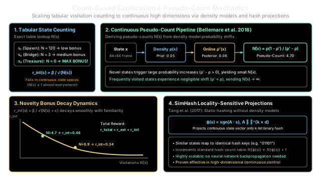
Why Does This Exist?

In sparse-reward reinforcement learning problems—such as navigating a labyrinth, solving Montezuma's Revenge, or discovering a robotic manipulation strategy—an agent relying solely on dithering strategies like $\epsilon$-greedy or Gaussian action noise faces an exponential sample complexity. Because extrinsic rewards $r_{\text{ext}}$ are zero almost everywhere, random motor twitching has a negligible probability of discovering the goal sequence.

In finite tabular Markov Decision Processes, the principle of Optimism in the Face of Uncertainty (OFU) solves this through Upper Confidence Bound (UCB) bonuses: states visited fewer times receive an intrinsic exploration incentive proportional to $N(s)^{-1/2}$, driving the agent systematically toward unvisited states.

However, classic visitation counting breaks catastrophically in continuous or high-dimensional state spaces (e.g., Atari pixel frames or continuous robot joint configurations). Because raw pixel observations or floating-point vectors are never revisited identically twice, the empirical visitation count is trivially $N(s) = 1$ for every encountered state. Without a generalization mechanism, standard tabular count-based methods collapse. Count-based exploration with pseudo-counts and locality-sensitive hashing exists to extend tabular exploration guarantees to high-dimensional and continuous domains by deriving generalized visitation frequencies from density models or spatial projections.

Think of It Like This

How It Actually Works

Tabular Count Bonuses to High-Dimensional Pseudo-Counts

In tabular environments, an agent maintains an exact state-action or state visitation counter $N(s)$. The total augmented reward presented to the reinforcement learning algorithm is:

where the intrinsic exploration bonus is governed by:

Here, $\beta > 0$ controls the exploration strength, and $c > 0$ prevents division by zero. By the upper confidence bound principle (e.g., in MBIE-EB or UCB1), this bonus ensures the agent seeks out states whose value estimates carry high epistemic uncertainty.

To scale this to continuous state spaces $\mathcal{S}$, Bellemare et al. (2016) introduced the pseudo-count derived from a sequential density model $\rho$. Let $\rho_t(x)$ denote the predictive probability of observing state $x$ given a history of states $x_{1:t}$, and let $\rho'_t(x) = \rho(x \mid x_{1:t} x)$ denote the updated predictive probability after recording an additional observation of $x$.

Under an idealized empirical count model with total steps $n$, observing state $x$ with empirical count $N_n(x)$ yields:

Solving this system of linear equations for the unknown state count $N_n(x)$ and total pseudo-sample size $n$ produces the pseudo-count $\hat{N}_n(x)$ and pseudo-gain $\hat{n}_n(x)$:

Whenever the density model is learning-positive (meaning observing $x$ strictly increases its future probability, $\rho'_n(x) > \rho_n(x)$), the pseudo-count $\hat{N}_n(x) \ge 0$ is well-defined and acts as a surrogate visitation frequency. The intrinsic reward bonus is then:

Locality-Sensitive Hashing (SimHash)

An alternative, computationally efficient approach to pseudo-counts in continuous state spaces is Locality-Sensitive Hashing (LSH) (Tang et al., 2017). A continuous state embedding $s \in \mathbb{R}^d$ is mapped to a discrete $k$-bit hash code via a random projection matrix $A \in \mathbb{R}^{k \times d}$ with entries drawn i.i.d. from $\mathcal{N}(0, 1)$:

Angular proximity between states is preserved: if two states are close in Euclidean space, the probability of them colliding into the exact same hash code $\phi(s)$ is proportional to $1 - \frac{\theta(s_1, s_2)}{\pi}$. The algorithm maintains a hash table of discrete bucket counts $N(\phi(s))$, updating:

Worked numerical example

Consider an agent exploring a 2D continuous environment evaluated with a predictive density model. We set exploration scale $\beta = 1.0$ and smoothing constant $c = 0.01$.

Step 1: First exposure to state $x_A$

• Before the observation, the density model assigns prior probability $\rho(x_A) = 0.05$.
• After conditioning on observing $x_A$, the updated density increases to $\rho'(x_A) = 0.06$.
• Compute the pseudo-count $\hat{N}(x_A)$:

• Compute the intrinsic exploration bonus:

• If the environment returns zero external reward ($r_{\text{ext}} = 0.0$), the augmented reward is $r_{\text{total}} = 0.0 + 0.4608 = 0.4608$.

Step 2: Re-visitation after multiple exposures

• After repeated passes through that corridor, the state has become familiar. The prior probability has risen to $\rho(x_A) = 0.10$.
• A further observation yields updated density $\rho'(x_A) = 0.11$.
• Re-compute the pseudo-count $\hat{N}(x_A)$:

• Compute the new intrinsic reward bonus:

• Notice the decay ratio:

The novelty bonus drops by $27.3\%$, motivating the policy to allocate attention to other regions whose pseudo-counts remain near zero.

Code

Below is a complete, self-contained implementation demonstrating both Bellemare pseudo-count derivation and SimHash-based count exploration for continuous states.

1from typing import Dict, Tuple, Union2import numpy as np3
4
5class BellemarePseudoCount:6    """Computes high-dimensional pseudo-counts from sequential density estimates."""7
8    def __init__(self, beta: float = 1.0, epsilon_smooth: float = 0.01) -> None:9        self.beta = beta10        self.epsilon_smooth = epsilon_smooth11
12    def compute_pseudo_count(self, rho: float, rho_prime: float) -> float:13        """Computes pseudo-count N_hat given prior and posterior densities.14
15        Formula: N_hat = rho * (1 - rho_prime) / (rho_prime - rho)16        """17        diff = rho_prime - rho18        if diff <= 1e-12:19            # If the model didn't gain confidence, novelty is treated as very high20            return 0.021        n_hat = (rho * (1.0 - rho_prime)) / diff22        return max(0.0, float(n_hat))23
24    def compute_bonus(self, n_hat: float) -> float:25        """Calculates exploration bonus: r_int = beta / sqrt(N_hat + c)."""26        bonus = self.beta / np.sqrt(n_hat + self.epsilon_smooth)27        return float(bonus)28
29
30class SimHashExploration:31    """Locality-Sensitive Hashing (SimHash) for continuous state count bonuses."""32
33    def __init__(34        self,35        state_dim: int,36        hash_bits: int = 16,37        beta: float = 1.0,38        seed: int = 42,39    ) -> None:40        self.state_dim = state_dim41        self.hash_bits = hash_bits42        self.beta = beta43        rng = np.random.default_rng(seed)44        # Random hyperplanes drawn from standard Gaussian: (k, d)45        self.projection_matrix = rng.standard_normal((hash_bits, state_dim))46        # Hash table recording visitation frequency per binary code47        self.counts: Dict[Tuple[int, ...], int] = {}48
49    def hash_state(self, state: np.ndarray) -> Tuple[int, ...]:50        """Projects continuous state vector into discrete binary hash code."""51        projected = self.projection_matrix @ state52        binary_code = tuple((projected >= 0).astype(int).tolist())53        return binary_code54
55    def step(self, state: np.ndarray) -> Tuple[float, int]:56        """Records state visitation, updates counter, and returns (bonus, count)."""57        code = self.hash_state(state)58        current_count = self.counts.get(code, 0) + 159        self.counts[code] = current_count60        bonus = self.beta / np.sqrt(current_count)61        return float(bonus), current_count62
63
64if __name__ == "__main__":65    # --- 1. Bellemare Pseudo-Count Verification ---66    bellemare = BellemarePseudoCount(beta=1.0, epsilon_smooth=0.01)67
68    # Step 1: Initial exposure (rho = 0.05 -> rho' = 0.06)69    n_hat_1 = bellemare.compute_pseudo_count(rho=0.05, rho_prime=0.06)70    bonus_1 = bellemare.compute_bonus(n_hat_1)71    print(f"Observation 1 -> N_hat: {n_hat_1:.2f}, Bonus: {bonus_1:.4f}")72    assert np.isclose(n_hat_1, 4.70), f"Expected 4.70, got {n_hat_1}"73    assert np.isclose(bonus_1, 0.4608, atol=1e-4), f"Expected 0.4608, got {bonus_1}"74
75    # Step 2: Familiar state (rho = 0.10 -> rho' = 0.11)76    n_hat_2 = bellemare.compute_pseudo_count(rho=0.10, rho_prime=0.11)77    bonus_2 = bellemare.compute_bonus(n_hat_2)78    print(f"Observation 2 -> N_hat: {n_hat_2:.2f}, Bonus: {bonus_2:.4f}")79    assert np.isclose(n_hat_2, 8.90), f"Expected 8.90, got {n_hat_2}"80    assert np.isclose(bonus_2, 0.3350, atol=1e-4), f"Expected 0.3350, got {bonus_2}"81
82    # Decay ratio verification83    decay = bonus_2 / bonus_184    print(f"Bonus Decay Factor: {decay:.4f}")85    assert np.isclose(decay, 0.7270, atol=1e-3), f"Expected ~0.7270, got {decay}"86
87    # --- 2. SimHash Continuous State Exploration ---88    simhash = SimHashExploration(state_dim=4, hash_bits=8, beta=1.0, seed=1337)89
90    # State A (e.g. spawn zone) visited multiple times91    state_a = np.array([0.5, -0.2, 1.1, -0.8])92    bonus_a1, count_a1 = simhash.step(state_a)93    bonus_a2, count_a2 = simhash.step(state_a)94    bonus_a3, count_a3 = simhash.step(state_a)95
96    print(f"State A visit 1 -> Count: {count_a1}, Bonus: {bonus_a1:.4f}")97    print(f"State A visit 2 -> Count: {count_a2}, Bonus: {bonus_a2:.4f}")98    print(f"State A visit 3 -> Count: {count_a3}, Bonus: {bonus_a3:.4f}")99
100    # State B (novel distant zone) visited for the first time101    state_b = np.array([-1.8, 2.4, -0.5, 3.1])102    bonus_b1, count_b1 = simhash.step(state_b)103    print(f"State B visit 1 -> Count: {count_b1}, Bonus: {bonus_b1:.4f}")104
105    assert count_a3 == 3106    assert bonus_a3 == 1.0 / np.sqrt(3.0)107    assert count_b1 == 1108    assert bonus_b1 == 1.0  # Novel state receives maximum exploration incentive109    print("All count-based exploration assertions passed successfully!")

1Observation 1 -> N_hat: 4.70, Bonus: 0.46082Observation 2 -> N_hat: 8.90, Bonus: 0.33503Bonus Decay Factor: 0.72704State A visit 1 -> Count: 1, Bonus: 1.00005State A visit 2 -> Count: 2, Bonus: 0.70716State A visit 3 -> Count: 3, Bonus: 0.57747State B visit 1 -> Count: 1, Bonus: 1.00008All count-based exploration assertions passed successfully!

Watch Out For

The Quick Version

• Extending tabular bounds: Count-based exploration generalizes the tabular upper confidence bound bonus $r_{\text{int}} \propto 1/\sqrt{N(s)}$ to continuous high-dimensional spaces where exact states are never visited twice.
• Pseudo-counts from density models: Bellemare's pseudo-count $\hat{N}_n(x) = \frac{\rho(x)(1 - \rho'(x))}{\rho'(x) - \rho(x)}$ deduces effective visitation counts from the change in predictive probability assigned by a density model before and after observing the state.
• Locality-Sensitive Hashing (SimHash): Random hyperplanes project continuous state vectors into discrete bit vectors $\phi(s) = \operatorname{sgn}(As)$, allowing standard hash-table counting over angularly similar geometric clusters.
• Bonus decay and extinction: Intrinsic rewards naturally decay as unfamiliar states become familiar, eventually allowing extrinsic task rewards to dominate the agent's long-term value function.
• Representation sensitivity: Applying pseudo-counts directly to raw pixels causes agents to become trapped by environmental noise (the "noisy TV" trap); learned or invariant latent embeddings are required in visually complex domains.

What to Read Next

• Exploration vs. Exploitation
• Upper Confidence Bound (UCB)
• Noisy Nets for Exploration