Noisy Nets for Exploration
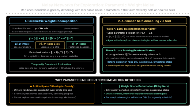
Noisy Nets inject learnable parametric noise into neural network weights, driving state-dependent exploration that automatically self-anneals as learning progresses.
Why Does This Exist?
In classic deep reinforcement learning, agents rely on heuristic -greedy exploration: with probability , the agent selects the greedy action , and with probability , it samples a uniformly random action from .
While simple, -greedy suffers from three critical deficiencies:
- Destructive Action Dithering: -greedy explores in action space by sampling independent random choices at every single time step. This introduces Brownian random-walk dynamics: the agent moves left, then right, then left, canceling its own progress. In environments requiring coherent multi-step navigation (such as navigating a maze or solving sparse-reward games like Montezuma's Revenge), random dithering virtually never reaches distant goals.
- State-Agnostic Exploration: -greedy treats every state identically. Even after an agent has completely mastered opening moves, it continues executing random, game-ending blunders with probability .
- Brittle Hyperparameter Schedules: Designing an exploration schedule requires manually tuning , , and decay rates across millions of frames, which rarely transfers across different tasks.
Introduced by Meire Fortunato et al. (DeepMind, 2018), Noisy Networks for Exploration (Noisy Nets) replace heuristic action dithering with learnable parametric noise injected directly into the neural network's weights. By perturbing parameters rather than actions, the policy remains temporally consistent across consecutive decisions, enabling structured, deep exploration.
Crucially, because the noise scale parameters are updated by gradient descent, exploration naturally self-anneals: as value uncertainty declines in mastered states, gradients automatically drive .
Think of It Like This
The Trembling Hands of a Novice Musician
Imagine an aspiring student learning to play acoustic guitar or violin.
If the student practiced using -greedy exploration, they would play nine notes with textbook precision, but on every tenth note, an involuntary muscle spasm would cause them to strike an unrelated string or drop the bow entirely. That abrupt action dithering does not teach acoustic subtlety—it merely derails the melody and destroys musical rhythm.
With Noisy Nets (parametric weight noise), the exploration originates internally within the motor cortex. During early practice, the student's grip, wrist tension, and finger pressure are slightly unsteady ( is large). This continuous tremor subtly alters vibrato, fretboard angle, and string contact across entire musical phrases. Because the variation is integrated directly into their motor coordination, the student discovers resonant harmonics, alternative fingerings, and dynamic expression.
As muscle memory consolidates and auditory feedback confirms pitch accuracy, the motor cortex naturally tightens control: the tremor variance dampens toward zero on mastered chords. However, when the student encounters an unfamiliar, complex chord progression in a minor key, flexibility naturally re-emerges to search for optimal finger placement.
Where the analogy stops: Human muscle tremor is physical biomechanics. In Noisy Nets, the tremor is precisely factorised Gaussian noise sampled on network forward passes and modulated by mathematical backpropagation gradients.
How It Actually Works
Mathematical Formulation and Factorised Noise Architecture
In a standard deterministic fully-connected layer, an input vector is transformed to output via:
Where and are learnable parameter tensors.
A NoisyLinear layer replaces fixed weights and biases with random variables parameterized by learnable means () and learnable noise scale deviations ():
Where:
- and are learnable mean parameters.
- and are learnable noise scale parameters.
- and are zero-mean stochastic noise tensors.
- denotes element-wise (Hadamard) multiplication.
Independent vs. Factorised Gaussian Noise
There are two primary ways to generate the noise tensors and :
-
Independent Gaussian Noise: Every element and is sampled independently from . This requires generating random variables per forward pass, which becomes computationally prohibitive in deep networks with wide hidden layers.
-
Factorised Gaussian Noise (Standard in Deep RL): Instead of generating independent variables, factorised noise generates only unit Gaussian variables for the inputs () and variables for the outputs (), requiring only random draws.
Each component is transformed using the non-linear real-valued function:
The weight and bias noise matrices are then constructed via outer product:
The Self-Annealing Gradient Mechanism
During backpropagation, gradients flow into both the mean parameters and the scale parameters:
Why does exploration self-anneal? Consider a state where the agent has already converged to the correct value function. In this regime, weight perturbations cause the network's output to deviate from the optimal Bellman target, increasing the loss . Because the gradient is positively correlated with loss increases, gradient descent pushes downward toward zero.
In contrast, in novel states with high value uncertainty, exploratory perturbations uncover rewarding trajectories that reduce the loss, sustaining non-zero values. The network autonomously decides where and how much to explore without manual schedules.
Worked Numerical Example
Consider a single NoisyLinear neuron with inputs and output.
Step 1: Initial Parameters and Input
- Input vector:
- Mean parameters: ,
- Scale parameters: ,
- Learning rate:
Step 2: Factorised Noise Generation
- Sample input noise:
- Sample output noise:
Apply transform :
Compute noise matrices:
Step 3: Realized Weights and Forward Pass
Realize perturbed parameters:
Compute perturbed forward output:
(Note: The deterministic unperturbed mean output is . Parametric noise shifted the output by .)
Step 4: Loss and Gradient Backpropagation
Suppose the target Bellman value is .
- Loss:
- Output error:
Compute parameter gradients:
Step 5: SGD Parameter Update ()
The Self-Annealing Effect in Action: Because the positive noise perturbation caused the network to significantly overshoot the target ( vs. ), gradient descent directly reduced the noise scale parameters:
- decreased from
- decreased from
- decreased from
The layer autonomously dampened its noise parameters to restore precision.
Code
import mathimport randomfrom typing import List, Sequence, Tuple
def f_transform(x: float) -> float: """Factorised noise non-linear transform: f(x) = sgn(x) * sqrt(|x|).""" return math.copysign(math.sqrt(abs(x)), x)
class NoisyLinear: """Fully-connected layer with factorised Gaussian parametric noise."""
def __init__(self, in_features: int, out_features: int, sigma_zero: float = 0.5) -> None: self.in_features = in_features self.out_features = out_features
# Initialize mean parameters (mu) and scale parameters (sigma) bound = 1.0 / math.sqrt(in_features) self.mu_w: List[List[float]] = [ [random.uniform(-bound, bound) for _ in range(in_features)] for _ in range(out_features) ] self.mu_b: List[float] = [random.uniform(-bound, bound) for _ in range(out_features)]
sigma_w_init = sigma_zero / math.sqrt(in_features) self.sigma_w: List[List[float]] = [ [sigma_w_init for _ in range(in_features)] for _ in range(out_features) ] self.sigma_b: List[float] = [ sigma_zero / math.sqrt(out_features) for _ in range(out_features) ]
# Internal noise buffers self.eps_in: List[float] = [0.0] * in_features self.eps_out: List[float] = [0.0] * out_features
def sample_noise( self, eps_in: Sequence[float] | None = None, eps_out: Sequence[float] | None = None, ) -> None: """Sample or inject factorised Gaussian noise.""" if eps_in is not None and eps_out is not None: self.eps_in = list(eps_in) self.eps_out = list(eps_out) else: self.eps_in = [random.gauss(0.0, 1.0) for _ in range(self.in_features)] self.eps_out = [random.gauss(0.0, 1.0) for _ in range(self.out_features)]
def forward(self, x: Sequence[float]) -> List[float]: """Compute y = (mu_w + sigma_w * eps_w) x + (mu_b + sigma_b * eps_b).""" f_in = [f_transform(v) for v in self.eps_in] f_out = [f_transform(v) for v in self.eps_out]
outputs = [0.0] * self.out_features for i in range(self.out_features): b_realized = self.mu_b[i] + self.sigma_b[i] * f_out[i] w_dot_x = 0.0 for j in range(self.in_features): weight_noise = f_out[i] * f_in[j] w_realized = self.mu_w[i][j] + self.sigma_w[i][j] * weight_noise w_dot_x += w_realized * x[j] outputs[i] = w_dot_x + b_realized
return outputs
if __name__ == "__main__": # Reproduce the exact worked numerical example (p=2 inputs, q=1 output) layer = NoisyLinear(in_features=2, out_features=1)
# Set parameters to exact test values layer.mu_w[0] = [0.5, -0.2] layer.mu_b[0] = 0.1 layer.sigma_w[0] = [0.4, 0.3] layer.sigma_b[0] = 0.2
# Inject exact factorised noise vectors layer.sample_noise(eps_in=[1.0, -4.0], eps_out=[1.0])
x = [2.0, -1.0] y = layer.forward(x)[0] print(f"Forward Output y: {y:.4f}")
# Compute loss against target y* = 1.50 y_star = 1.50 delta = y - y_star loss = 0.5 * (delta**2) print(f"Target: {y_star:.2f}, Delta: {delta:.4f}, Loss: {loss:.4f}")
# Compute analytical gradients f_in = [f_transform(v) for v in layer.eps_in] f_out = [f_transform(v) for v in layer.eps_out] eps_w = [f_out[0] * f_in[0], f_out[0] * f_in[1]] eps_b = f_out[0]
grad_mu_w = [delta * x[j] for j in range(2)] grad_sigma_w = [delta * x[j] * eps_w[j] for j in range(2)] grad_mu_b = delta grad_sigma_b = delta * eps_b
print(f"Grad mu_w: {[round(g, 4) for g in grad_mu_w]}") print(f"Grad sigma_w: {[round(g, 4) for g in grad_sigma_w]}") print(f"Grad mu_b: {grad_mu_b:.4f}") print(f"Grad sigma_b: {grad_sigma_b:.4f}")
# Apply SGD parameter update with learning rate alpha = 0.1 lr = 0.1 layer.mu_w[0] = [layer.mu_w[0][j] - lr * grad_mu_w[j] for j in range(2)] layer.sigma_w[0] = [layer.sigma_w[0][j] - lr * grad_sigma_w[j] for j in range(2)] layer.mu_b[0] -= lr * grad_mu_b layer.sigma_b[0] -= lr * grad_sigma_b
print("\nUpdated Parameters after 1 Step:") print(f"mu_w: {[round(v, 4) for v in layer.mu_w[0]]}") print(f"sigma_w: {[round(v, 4) for v in layer.sigma_w[0]]}") print(f"mu_b: {layer.mu_b[0]:.4f}") print(f"sigma_b: {layer.sigma_b[0]:.4f}")# Expected Output:# Forward Output y: 2.9000# Target: 1.50, Delta: 1.4000, Loss: 0.9800# Grad mu_w: [2.8, -1.4]# Grad sigma_w: [2.8, 2.8]# Grad mu_b: 1.4000# Grad sigma_b: 1.4000# # Updated Parameters after 1 Step:# mu_w: [0.22, -0.06]# sigma_w: [0.12, 0.02]# mu_b: -0.0400# sigma_b: 0.0600Watch Out For
The Step-Level Noise Resampling Trap
A frequent mistake when integrating Noisy Nets into deep Q-networks is resampling the noise tensors at every single environment decision step.
If you draw fresh noise vectors on every individual time step, parameter space noise collapses into high-frequency Brownian dithering. The agent acts on a different set of perturbed weights every fraction of a second, destroying the temporally extended trajectories that make Noisy Nets effective.
The Fix: Resample the noise tensors and strictly once per environment step (or once per episode in actor-critic setups), keeping the realized weights frozen while computing Q-values across all discrete action candidates for the current state. During training, sample a new set of noise for each sampled mini-batch to compute the Bellman error gradient.
The Quick Version
- Weight Space Exploration: Replaces heuristic -greedy action dithering by injecting stochastic noise directly into neural network weights ().
- Temporally Consistent Policies: Because parameters remain stable across decision evaluations, the agent executes coherent multi-step exploratory sequences rather than random Brownian jitter.
- Autonomous Self-Annealing: Gradients naturally penalize noise scale parameters in mastered states where perturbations increase Bellman loss, driving without manual decay schedules.
- Factorised Efficiency: Factorised Gaussian noise generates weight perturbations via outer products of input and output vectors (), reducing noise variables from down to .