Covariance Matrix Adaptation Evolution Strategy (CMA-ES)

Why Does This Exist?

Some problems give you no usable gradient. The simulator is not differentiable, the reward arrives as a single score at the end of an episode, or the surface is discontinuous, so stochastic gradient descent in RL has nothing to differentiate. That is exactly where policy search lives: you try whole parameter vectors, score each rollout, and keep what works. Policy gradient methods do this with estimated gradients, but they still assume you can get a reliable gradient signal from those scores.

Plain evolution strategies fill the gap with a fixed sampling cloud: draw candidates around a mean, keep the best, move the mean. That works on round, well-scaled problems and stalls on stretched ones. Picture tuning a robot controller where one gain is a hundred times more sensitive than another, or a narrow curved valley like a Rosenbrock function. A spherical cloud wastes nearly every sample on directions that fail, and a hand-picked step size is either too timid along the valley or too wild across it.

CMA-ES, introduced by Hansen and Ostermeier, removes both hand choices. It learns the full shape of the cloud (the covariance) and its global scale (the step size) from the history of successful steps. This page teaches that adaptation loop: the sampling rule, the weighted mean move, the two-part covariance update, the step-size test, and the invariances you get for free. For the sampling spread question in general, see exploration vs exploitation.

Think of It Like This

How It Actually Works

CMA-ES keeps one search distribution and updates it every generation:

$x = m + \sigma C^{1/2} z, \quad z \sim \mathcal{N}(0, I)$

• $m$ is the mean vector, the center of the cloud and the current best guess.
• $\sigma > 0$ is the step size, one global scale factor for every direction.
• $C$ is the covariance matrix, a symmetric positive-definite matrix whose eigenvectors set the ellipse axes and whose eigenvalues set their squared lengths.
• $z$ is a standard normal draw, reshaped by $C^{1/2}$ and scaled by $\sigma$ into a candidate $x$.

Each generation samples $\lambda$ candidates, scores each with the fitness function $f$ (lower is better by convention here), sorts them best first as $x_{1:\lambda}, \dots, x_{\lambda:\lambda}$, and keeps the top $\mu$ with fixed weights $w_1 \ge w_2 \ge \dots \ge w_\mu > 0$ summing to 1. Only the ranking matters, never the raw scores.

One mean update, computed by hand

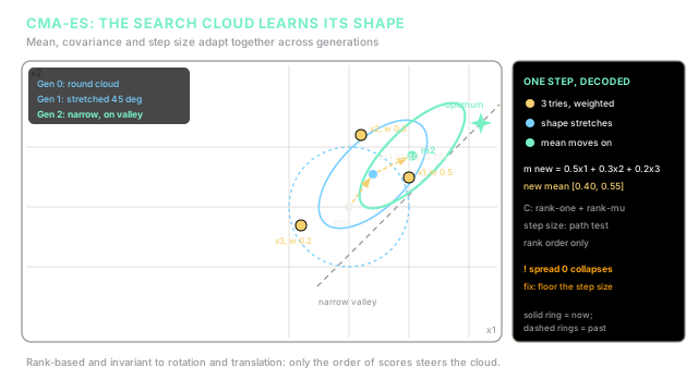
Start at $m = [0, 0]$ with $\sigma = 1$ and $C = I$ (a round cloud). Three samples come back ranked best first:

• $x_1 = [1.0, 0.5]$, weight $w_1 = 0.5$
• $x_2 = [0.2, 1.2]$, weight $w_2 = 0.3$
• $x_3 = [-0.8, -0.3]$, weight $w_3 = 0.2$

The new mean is the weighted recombination:

$m' = \sum_{i=1}^{3} w_i x_{i:3}$

First coordinate: $0.5 \times 1.0 + 0.3 \times 0.2 + 0.2 \times (-0.8) = 0.50 + 0.06 - 0.16 = 0.40$.

Second coordinate: $0.5 \times 0.5 + 0.3 \times 1.2 + 0.2 \times (-0.3) = 0.25 + 0.36 - 0.06 = 0.55$.

So $m' = [0.40, 0.55]$. The mean steps toward the good half of the cloud but keeps a pull from every keeper, which steadies it against one lucky draw. The effective selection mass here is $\mu_{\text{eff}} = 1 / (0.5^2 + 0.3^2 + 0.2^2) = 1 / 0.38 \approx 2.63$, so this generation counts as roughly two and a half independent winners.

How the covariance learns direction

Write each keeper as a scaled step from the old mean: $y_i = (x_{i:\lambda} - m) / \sigma$. The covariance update blends three terms:

$C' = (1 - c_1 - c_\mu) C + c_1 p_c p_c^T + c_\mu \sum_{i=1}^{\mu} w_i y_i y_i^T$

• The rank-$\mu$ term (rightmost sum) stretches $C$ along this generation's winning steps. Many winners pointing northeast fattens the ellipse toward the northeast.
• The rank-one term ($p_c p_c^T$) stretches $C$ along the evolution path $p_c$, a fading average of recent mean moves: $p_c' = (1 - c_c) p_c + \sqrt{c_c (2 - c_c) \mu_{\text{eff}}} \, (m' - m) / \sigma$. It notices when steps agree across generations even if no single generation looks stretched.
• $c_1$, $c_\mu$ and $c_c$ are small learning rates (typical $c_1 \approx 0.2 / n^2$ side values from the original papers for dimension $n$). Small values keep $C$ positive-definite and stop one odd generation from collapsing the cloud.

In the diagram, the round Gen 0 ring becomes the tilted Gen 1 ellipse and then the narrow Gen 2 ellipse riding the valley. Same idea, drawn to our numbers for the mean and the samples.

How the step size learns pace

A second path $p_\sigma$ tracks consecutive mean moves, normalized so its length under pure random selection averages $E\lVert \mathcal{N}(0, I) \rVert$ (about $1.25$ in two dimensions). The step size follows:

$\sigma' = \sigma \exp\left(\frac{c_\sigma}{d_\sigma} \left(\frac{\lVert p_\sigma \rVert}{E\lVert \mathcal{N}(0, I) \rVert} - 1\right)\right)$

Steps that march one way grow $\lVert p_\sigma \rVert$ past the baseline, so $\sigma$ grows and the cloud strides. Steps that cancel shrink it, so $\sigma$ tightens and the cloud fine-tunes. $c_\sigma$ sets how fast $\sigma$ reacts and $d_\sigma$ damps the change.

Why practitioners trust it: three invariances

• Translation invariant: only differences $x - m$ enter the updates, so shifting the whole problem changes nothing.
• Rotation invariant: $C$ learns orientation, so a rotated valley costs the same as an axis-aligned one. Fixed-shape methods can differ by orders of magnitude here.
• Order invariant: weights depend on ranks, so any strictly increasing transform of $f$ gives identical behavior. Rescaling rewards mid-tuning cannot break it.

The price is sample cost: the default population grows like $4 + 3 \ln n$ with dimension $n$, and learning a full $n \times n$ covariance needs on the order of $n^2$ samples. Past a few hundred dimensions, use a restricted variant (separable or limited-memory CMA-ES) instead.

Code

A minimal weighted-mean step in pure Python, using the worked numbers above:

1from typing import List, Tuple2
3samples: List[Tuple[float, float]] = [(1.0, 0.5), (0.2, 1.2), (-0.8, -0.3)]4weights: List[float] = [0.5, 0.3, 0.2]5
6mean_x = sum(w * x for w, (x, _) in zip(weights, samples))7mean_y = sum(w * y for w, (_, y) in zip(weights, samples))8mu_eff = 1.0 / sum(w * w for w in weights)9
10print(f"new mean: [{mean_x:.2f}, {mean_y:.2f}]")11print(f"effective winners: {mu_eff:.2f}")12print(f"weights sum to: {sum(weights):.1f}")

1# -> expected output:2new mean: [0.40, 0.55]3effective winners: 2.634weights sum to: 1.0

Watch Out For

The Quick Version

• CMA-ES samples candidates from one Gaussian $m + \sigma C^{1/2} z$ and moves $m$ to the weighted average of the top-ranked tries, as in $[0.40, 0.55]$ from weights $[0.5, 0.3, 0.2]$.
• The covariance update pairs a rank-$\mu$ term that stretches along this generation's winners with a rank-one term that stretches along the multi-generation evolution path.
• The step size $\sigma$ grows when successive mean moves point one way and shrinks when they cancel, judged against the expected random-selection path length.
• Ranking-only selection makes it invariant to any increasing rescaling of fitness, plus translation and rotation invariant by construction.
• It needs no gradients, which suits non-differentiable simulators and episodic policy scores, but full covariance learning costs on the order of $n^2$ samples in dimension $n$.

What to Read Next

• Stochastic Gradient Descent in RL
• Exploration vs. Exploitation
• Policy Gradient Methods