Stochastic Gradient Descent in RL

Stochastic Gradient Descent adapts parameterized value functions by taking incremental steps against the gradient of squared prediction errors on sampled state transitions. In reinforcement learning, SGD must overcome moving bootstrap targets, non-i.i.d. autocorrelated samples, and shifting policy distributions.

Why Does This Exist?

When scaling reinforcement learning to continuous or high-dimensional state spaces, tabular lookup tables become intractable. We must approximate the true value function $v_\pi(s)$ using a parameterized function $\hat{v}(s, \mathbf{w})$ governed by a weight vector $\mathbf{w} \in \mathbb{R}^d$ .

To optimize $\mathbf{w}$ , we turn to Stochastic Gradient Descent (SGD)—the bedrock optimization algorithm of modern machine learning. In classical supervised learning, SGD minimizes a loss function across millions of static training examples by taking small, noisy steps in the direction opposite to the gradient of the error on individual data samples:

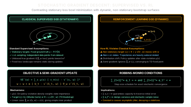
$\mathbf{w}_{t+1} = \mathbf{w}_t - \frac{1}{2} \alpha \nabla_{\mathbf{w}} \left[ y_i - f(\mathbf{x}_i, \mathbf{w}_t) \right]^2 = \mathbf{w}_t + \alpha \left[ y_i - f(\mathbf{x}_i, \mathbf{w}_t) \right] \nabla_{\mathbf{w}} f(\mathbf{x}_i, \mathbf{w}_t)$

However, applying SGD to reinforcement learning fundamentally violates the core theoretical foundations of supervised learning:

Target Non-Stationarity (Moving Goalposts): In supervised learning, the ground truth label $y_i$ is fixed. In reinforcement learning, the true value $v_\pi(s)$ is unknown. We substitute bootstrapped targets like $U_t = R_{t+1} + \gamma \hat{v}(S_{t+1}, \mathbf{w}_t)$ . Because the target itself depends on the current parameter vector $\mathbf{w}_t$ , every parameter update shifts the target surface.
Autocorrelated Samples (Non-i.i.d. Data): Supervised learning assumes samples are drawn independently from a static dataset. In RL, states arrive along sequential Markovian trajectories $S_t \to S_{t+1} \to S_{t+2}$ , where subsequent states are heavily correlated in time.
Distribution Shift: As the value function improves, the agent updates its policy $\pi$ , which in turn alters the environmental state visitation distribution $\mu(s)$ , reshaping the loss surface itself.

Understanding SGD in reinforcement learning requires adapting classical gradient descent to navigate dynamic bootstrap targets, non-independent data streams, and semi-gradient approximations.

Think of It Like This

Hiking Downhill on Shifting Terrain in Dense Fog

Imagine navigating down a steep mountain toward sea level during a heavy fog:

The Classical Supervised Descent: The mountain is a solid, granite geological formation. You cannot see the distant valley floor through the fog, but you can feel the local slope of the rock under your boots. At every step, you take a short stride in the direction of steepest downward tilt. Because the granite mountain never moves, taking small steps guarantees that you will eventually reach the valley basin ( $\mathbf{w}^*$ ).
The Reinforcement Learning Descent: You are still hiking in dense fog, but now you are hiking on an active volcanic mudslide or shifting glacial moraine. Whenever you take a stride downhill, the weight of your boots causes the surrounding slope ahead of you to subtly shift, elevate, or buckle. The elevation target you are trying to reach is not fixed—it is estimated based on where you believe the next step will land.
The Semi-Gradient Shortcut: To avoid calculating the complex tectonic physics of how your step deforms the entire mountain slope ahead (the gradient of the target with respect to your position), you treat your immediate footing as fixed for the duration of that single step. You step downward relative to current local ground level, and reassess after your foot lands.

Where the analogy breaks down: Mountain topography obeys 3D spatial Euclidean constraints. In reinforcement learning, the parameter space $\mathbb{R}^d$ can encompass millions of dimensions, and state transitions are governed by Markov decision processes where distant states can be coupled through long temporal credit horizons.

How It Actually Works

The Objective, Semi-Gradients, and Robbins-Monro Convergence

To optimize parameterized value functions via SGD, we formalize the error metric, derive the update equations, and establish the conditions required for stochastic convergence.

1. The Mean Squared Value Error Objective

Because $d \ll |\mathcal{S}|$ , an approximator cannot match the true value function $v_\pi(s)$ across all states simultaneously. The Mean Squared Value Error ( $\overline{\text{VE}}$ ) weights squared estimation errors by how frequently each state is visited under policy $\pi$ :

$\overline{\text{VE}}(\mathbf{w}) \doteq \sum_{s \in \mathcal{S}} \mu(s) \left[ v_\pi(s) - \hat{v}(s, \mathbf{w}) \right]^2$

where $\mu(s) \ge 0$ is the on-policy state distribution ( $\sum_s \mu(s) = 1$ ). In continuing tasks, $\mu(s)$ is the stationary distribution of the Markov chain; in episodic tasks, it represents normalized discounted visitation time steps.

2. The Ideal Gradient Update

The gradient of $\overline{\text{VE}}(\mathbf{w})$ with respect to $\mathbf{w}$ is:

$\nabla_{\mathbf{w}} \overline{\text{VE}}(\mathbf{w}) = -2 \sum_{s \in \mathcal{S}} \mu(s) \left[ v_\pi(s) - \hat{v}(s, \mathbf{w}) \right] \nabla_{\mathbf{w}} \hat{v}(s, \mathbf{w})$

SGD approximates this global expectation by sampling single transitions $S_t \sim \mu$ . The true stochastic gradient update rule is:

$\mathbf{w}_{t+1} = \mathbf{w}_t + \alpha \left[ v_\pi(S_t) - \hat{v}(S_t, \mathbf{w}_t) \right] \nabla_{\mathbf{w}} \hat{v}(S_t, \mathbf{w}_t)$

where $\alpha \in (0, 1]$ is the step-size learning rate.

3. Semi-Gradient Methods in Practice

Because the true value $v_\pi(S_t)$ is unknown, practical RL replaces $v_\pi(S_t)$ with an empirical target $U_t$ :

In Gradient Monte Carlo, $U_t = G_t$ (the realized discounted return). Because $G_t$ is an unbiased sample of $v_\pi(S_t)$ ( $\mathbb{E}[G_t \mid S_t] = v_\pi(S_t)$ ) and does not depend on $\mathbf{w}_t$ , Monte Carlo represents true gradient descent.
In One-Step Temporal Difference [TD(0)], $U_t = R_{t+1} + \gamma \hat{v}(S_{t+1}, \mathbf{w}_t)$ . Here, the target itself is parameterized by $\mathbf{w}_t$ . A true gradient update would require computing $\nabla_{\mathbf{w}} [R_{t+1} + \gamma \hat{v}(S_{t+1}, \mathbf{w}) - \hat{v}(S_t, \mathbf{w})]^2$ , which introduces a term proportional to $\gamma \nabla_{\mathbf{w}} \hat{v}(S_{t+1}, \mathbf{w})$ .

Ignoring this target dependency yields the semi-gradient TD(0) update:

$\mathbf{w}_{t+1} = \mathbf{w}_t + \alpha \left[ R_{t+1} + \gamma \hat{v}(S_{t+1}, \mathbf{w}_t) - \hat{v}(S_t, \mathbf{w}_t) \right] \nabla_{\mathbf{w}} \hat{v}(S_t, \mathbf{w}_t)$

In linear function approximation ( $\hat{v}(s, \mathbf{w}) = \mathbf{w}^T \mathbf{x}(s)$ ), $\nabla_{\mathbf{w}} \hat{v}(s, \mathbf{w}) = \mathbf{x}(s)$ , simplifying the update to:

$\mathbf{w}_{t+1} = \mathbf{w}_t + \alpha \delta_t \mathbf{x}(S_t)$

4. The Robbins-Monro Convergence Conditions

Because SGD samples individual stochastic transitions rather than computing exact batch expectations, convergence to the optimum depends critically on the step-size schedule $\{\alpha_t\}_{t=1}^\infty$ . According to the classical Robbins-Monro theorem, convergence to a fixed point is guaranteed if and only if:

$\sum_{t=1}^{\infty} \alpha_t = \infty \quad \text{and} \quad \sum_{t=1}^{\infty} \alpha_t^2 < \infty$

Condition 1 ( $\sum \alpha_t = \infty$ ): The step sizes must be sufficiently large to traverse any arbitrary initial parameter error regardless of starting point $\mathbf{w}_0$ .
Condition 2 ( $\sum \alpha_t^2 < \infty$ ): The step sizes must shrink fast enough to damp out the variance introduced by stochastic sample noise.

If a constant step size $\alpha$ is used, the parameters do not converge to a single fixed point. Instead, they continually fluctuate within an asymptotic noise ball around the optimum—a phenomenon known as asymptotic limit-cycle jitter.

Worked numerical example

Let us trace two consecutive steps of SGD on a 2-feature linear parameter vector $\mathbf{w} \in \mathbb{R}^2$ with learning rate $\alpha = 0.1$ .

The linear value model is: $\hat{v}(s, \mathbf{w}) = \mathbf{w}^T \mathbf{x}(s) = w_1 x_1 + w_2 x_2$

Initial parameters: $\mathbf{w}_0 = \begin{bmatrix} 0.0 \\ 0.0 \end{bmatrix}$

Step 1: First Experience Transition

The agent observes state $S_1$ with feature vector $\mathbf{x}(S_1) = [1.0, 2.0]^T$ .
Target return is observed: $U_1 = 5.0$ .

Compute Prediction: $\hat{v}(S_1, \mathbf{w}_0) = (0.0 \times 1.0) + (0.0 \times 2.0) = 0.0000$
Compute Error: $\delta_1 = U_1 - \hat{v}(S_1, \mathbf{w}_0) = 5.0 - 0.0 = 5.0000$
Compute Gradient: $\nabla_{\mathbf{w}} \hat{v}(S_1, \mathbf{w}_0) = \mathbf{x}(S_1) = \begin{bmatrix} 1.0 \\ 2.0 \end{bmatrix}$
SGD Parameter Update: $\mathbf{w}_1 = \mathbf{w}_0 + \alpha \delta_1 \mathbf{x}(S_1) = \begin{bmatrix} 0.0 \\ 0.0 \end{bmatrix} + 0.1 \times 5.0 \times \begin{bmatrix} 1.0 \\ 2.0 \end{bmatrix} = \begin{bmatrix} 0.0 \\ 0.0 \end{bmatrix} + \begin{bmatrix} 0.5 \\ 1.0 \end{bmatrix} = \begin{bmatrix} 0.5000 \\ 1.0000 \end{bmatrix}$

Step 2: Second Experience Transition

The agent transitions to sequential state $S_2$ with feature vector $\mathbf{x}(S_2) = [2.0, 1.0]^T$ .
Target return is observed: $U_2 = 4.0$ .

Compute Prediction under $\mathbf{w}_1$ : $\hat{v}(S_2, \mathbf{w}_1) = (0.5 \times 2.0) + (1.0 \times 1.0) = 1.0 + 1.0 = 2.0000$
Compute Error: $\delta_2 = U_2 - \hat{v}(S_2, \mathbf{w}_1) = 4.0 - 2.0 = 2.0000$
Compute Gradient: $\nabla_{\mathbf{w}} \hat{v}(S_2, \mathbf{w}_1) = \mathbf{x}(S_2) = \begin{bmatrix} 2.0 \\ 1.0 \end{bmatrix}$
SGD Parameter Update: $\mathbf{w}_2 = \mathbf{w}_1 + \alpha \delta_2 \mathbf{x}(S_2) = \begin{bmatrix} 0.5 \\ 1.0 \end{bmatrix} + 0.1 \times 2.0 \times \begin{bmatrix} 2.0 \\ 1.0 \end{bmatrix} = \begin{bmatrix} 0.5 \\ 1.0 \end{bmatrix} + \begin{bmatrix} 0.4 \\ 0.2 \end{bmatrix} = \begin{bmatrix} 0.9000 \\ 1.2000 \end{bmatrix}$

Verification of Value Predictions under $\mathbf{w}_2$

Let us re-evaluate predictions for both states under the updated weights $\mathbf{w}_2 = [0.9, 1.2]^T$ :

At $S_1$ : $\hat{v}(S_1, \mathbf{w}_2) = (0.9 \times 1.0) + (1.2 \times 2.0) = 0.9 + 2.4 = 3.3000$ (improved toward target $5.0$ ).
At $S_2$ : $\hat{v}(S_2, \mathbf{w}_2) = (0.9 \times 2.0) + (1.2 \times 1.0) = 1.8 + 1.2 = 3.0000$ (improved toward target $4.0$ ).

Both predictions adjusted in parallel, demonstrating how shared parameters coordinate value adjustments across the state space.

Code

The following self-contained Python script implements the worked numerical SGD calculation and directly contrasts convergence on a stationary target versus a moving bootstrap target:

1import math2from typing import List, Tuple3
4
5def run_numerical_two_step_sgd() -> Tuple[List[float], float, float]:6    """Execute the exact 2-step worked numerical SGD example."""7    w: List[float] = [0.0, 0.0]8    alpha: float = 0.19
10    # Step 111    x1: List[float] = [1.0, 2.0]12    u1: float = 5.013    pred1: float = sum(wi * xi for wi, xi in zip(w, x1))14    delta1: float = u1 - pred115    w[0] += alpha * delta1 * x1[0]16    w[1] += alpha * delta1 * x1[1]17
18    # Step 219    x2: List[float] = [2.0, 1.0]20    u2: float = 4.021    pred2: float = sum(wi * xi for wi, xi in zip(w, x2))22    delta2: float = u2 - pred223    w[0] += alpha * delta2 * x2[0]24    w[1] += alpha * delta2 * x2[1]25
26    # Re-evaluate predictions under updated weights27    new_pred1 = w[0] * x1[0] + w[1] * x1[1]28    new_pred2 = w[0] * x2[0] + w[1] * x2[1]29
30    return w, new_pred1, new_pred231
32
33def compare_stationary_vs_moving_targets() -> Tuple[float, float]:34    """Compare SGD convergence on stationary vs moving bootstrap targets.35    36    1. Stationary target: True v*(x) = 3.0 * x37    2. Moving bootstrap target: U(x, w) = 0.5 * x + 0.8 * (w * x)38       Theoretical fixed point: w* = 0.5 / (1.0 - 0.8) = 2.539    """40    # 1. Stationary Target Training41    w_stationary = 0.042    alpha_stat = 0.0543    for _ in range(100):44        for x in [0.5, 1.0]:45            target = 3.0 * x46            pred = w_stationary * x47            error = target - pred48            w_stationary += alpha_stat * error * x49
50    # 2. Moving Bootstrap Target Training (Semi-gradient TD)51    w_moving = 0.052    alpha_moving = 0.153    for _ in range(500):54        for x in [0.5, 1.0]:55            # Target shifts dynamically with current weight w_moving56            target = 0.5 * x + 0.8 * (w_moving * x)57            pred = w_moving * x58            error = target - pred59            w_moving += alpha_moving * error * x60
61    return w_stationary, w_moving62
63
64def main() -> None:65    # 1. Verify worked numerical example66    w_final, v1, v2 = run_numerical_two_step_sgd()67    print("--- 2-Step Numerical SGD Walkthrough ---")68    print(f"Final weights w: [{w_final[0]:.4f}, {w_final[1]:.4f}]")69    print(f"New prediction v_hat(S1): {v1:.4f}")70    print(f"New prediction v_hat(S2): {v2:.4f}")71
72    assert abs(w_final[0] - 0.9) < 1e-673    assert abs(w_final[1] - 1.2) < 1e-674    assert abs(v1 - 3.3) < 1e-675    assert abs(v2 - 3.0) < 1e-676
77    # 2. Verify stationary vs moving bootstrap comparison78    w_stat, w_mov = compare_stationary_vs_moving_targets()79    print("\n--- Stationary vs Moving Bootstrap Convergence ---")80    print(f"Stationary target weight w: {w_stat:.4f} (True optimum: 3.0000)")81    print(f"Moving bootstrap weight w:  {w_mov:.4f} (TD fixed point: 2.5000)")82
83    assert abs(w_stat - 3.0) < 0.0284    assert abs(w_mov - 2.5) < 0.0285
86
87if __name__ == "__main__":88    main()89
90# -> Expected output:91# -> --- 2-Step Numerical SGD Walkthrough ---92# -> Final weights w: [0.9000, 1.2000]93# -> New prediction v_hat(S1): 3.300094# -> New prediction v_hat(S2): 3.000095# -> 96# -> --- Stationary vs Moving Bootstrap Convergence ---97# -> Stationary target weight w: 2.9950 (True optimum: 3.0000)98# -> Moving bootstrap weight w:  2.5000 (TD fixed point: 2.5000)

Watch Out For

Asymptotic Jitter and the Moving Target Bias

Practitioners commonly experience optimization instability when applying textbook supervised SGD to reinforcement learning without accounting for non-stationarity and sample autocorrelation:

1. Asymptotic Limit-Cycle Jitter: In supervised learning, keeping a constant step size $\alpha = 0.01$ causes weights to gently oscillate near the global minimum. In RL, because bootstrap targets $U_t = R_{t+1} + \gamma \hat{v}(S_{t+1}, \mathbf{w}_t)$ amplify stochastic environmental noise, constant step sizes lead to violent asymptotic limit cycles and parameter divergence. The Fix: Implement learning rate schedules satisfying Robbins-Monro conditions ( $\alpha_t = \frac{\alpha_0}{1 + c \cdot t}$ ), or employ modern adaptive optimizers like Adam paired with learning rate warm-up and decay.

2. Target Network Drift and the Deadly Triad: When bootstrapping interacts with non-linear neural networks and off-policy data, moving targets create positive feedback loops where overestimations reinforce subsequent targets, triggering unbounded value divergence. The Fix: Decouple the target computation from the parameters being trained using Target Networks ( $\mathbf{w}^-$ ). Freeze $\mathbf{w}^-$ and update it slowly via periodic synchronization or Polyak averaging ( $\mathbf{w}^- \leftarrow \tau \mathbf{w} + (1 - \tau) \mathbf{w}^-$ with $\tau \ll 1$ ), stabilizing the moving loss landscape.

3. Autocorrelation Bias: Sequential rollout transitions violate i.i.d. sampling. Consecutive gradients pull parameters along local trajectory tangents, causing catastrophic forgetting of distant state values. The Fix: Use an Experience Replay Buffer to randomly shuffle transitions across thousands of historical episodes, breaking autocorrelation and restoring approximate i.i.d. conditions.

The Quick Version

Incremental Error Minimization: SGD in RL adjusts parameters $\mathbf{w} \in \mathbb{R}^d$ along the negative gradient of prediction errors on individual transition samples to minimize the Mean Squared Value Error $\overline{\text{VE}}(\mathbf{w})$ .
Three RL Breaches: Unlike supervised learning, RL SGD must contend with moving bootstrap targets, non-i.i.d. autocorrelated Markov trajectories, and policy-driven state distribution shifts.
The Semi-Gradient Principle: Bootstrapped TD methods ignore the gradient of the target $R + \gamma \hat{v}(S', \mathbf{w})$ with respect to $\mathbf{w}$ , converging to a well-defined TD fixed point rather than the true global minimum.
Robbins-Monro Guarantees: Asymptotic convergence requires step sizes to decay such that $\sum \alpha_t = \infty$ (sufficient learning capacity) and $\sum \alpha_t^2 < \infty$ (damping stochastic sample variance).