Eligibility Traces

Eligibility traces act as a fading short-term memory that records which states were recently visited, allowing a single reward to immediately credit past decisions without waiting for the episode to end.

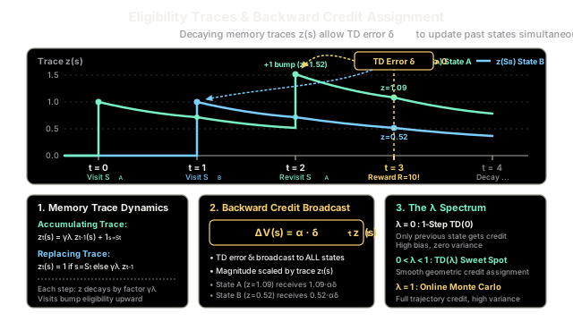
Why Does This Exist?

In multi-step decision problems, reinforcement learning faces the fundamental temporal credit assignment problem: when an agent receives a delayed reward after dozens of choices, which earlier actions actually caused the success?

Standard one-step temporal difference learning, $\text{TD}(0)$ , updates solely the single immediately preceding state $S_{t-1}$ . If a crucial choice was made ten steps before reaching a rewarding terminal state, information requires ten distinct, full traversals through that trajectory to trickle back to the source. Conversely, pure Monte Carlo methods update the entire sequence of visited states at once, but they require waiting until the episode terminates, cannot function in non-terminating continuing environments, and exhibit notoriously high variance.

Eligibility traces exist to bridge this gap. They provide an incremental, online backward-view mechanism that unifies one-step bootstrapping and multi-step Monte Carlo learning. By maintaining a decaying vector of state eligibilities $z_t \in \mathbb{R}^{|\mathcal{S}|}$ , a single one-step prediction error $\delta_t$ is instantly broadcast backward across every state that contributed to the current situation—achieving multi-step credit assignment on every single time step with minimal computational cost.

Think of It Like This

Footprints in the Sand and the Ocean Tide

Imagine walking across a sandy beach hunting for a buried treasure chest nestled among coastal dunes.

Every time you place a foot on the sand, you press a deep, fresh imprint into the shoreline. As the minutes tick by, ocean breezes and rising tides gently wash across the beach: your older footprints gradually soften and erode, while your most recent steps remain sharp and deep. If you circle back and step in the exact same spot twice, the indentation becomes even deeper.

The instant you unearth the gold chest, an aerial drone does not merely drop a celebratory reward on your final resting spot. Instead, it looks down at the entire coastline and scatters gold dust along your trail:

The freshest, deepest footprints right next to the chest receive the largest share of gold dust.
Footprints from five minutes earlier receive a moderate sprinkle.
Faint indentations from the start of your journey receive a small dusting.
Unvisited stretches of sand receive nothing at all.

Where the analogy breaks down: Real ocean tides erode footprints non-linearly depending on wind gusts and shoreline moisture. In reinforcement learning, eligibility traces decay strictly exponentially by a deterministic factor $(\gamma \lambda)$ on each discrete clock tick. Furthermore, tabular eligibility traces store a single scalar memory bucket per discrete state label rather than distinct spatial coordinates across continuous physical terrain.

How It Actually Works

The Eligibility Trace Vector and Decay Dynamics

An eligibility trace is an additional short-term memory variable associated with each state (or feature weight). We denote the eligibility trace vector at time step $t$ by $z_t \in \mathbb{R}^{|\mathcal{S}|}$ , initialized to zero at the beginning of an episode:

$z_0(s) = 0 \quad \forall s \in \mathcal{S}$

On every time step $t$ , two mathematical operations modify the trace vector:

Decay: All existing state traces decay exponentially by the product of the environmental discount factor $\gamma \in [0, 1]$ and the trace-decay parameter $\lambda \in [0, 1]$ : $\text{decay factor} = \gamma \lambda$
Visit Activation: The state visited at time $t$ , $S_t$ , receives an eligibility bump indicating its recency.

Practitioners commonly distinguish two classic formulation styles for tabular traces:

1. Accumulating Traces

In accumulating traces, every visit to state $s$ adds $+1$ directly to the trace without bound:

$z_t(s) = \begin{cases} \gamma \lambda z_{t-1}(s) + 1 & \text{if } s = S_t \\ \gamma \lambda z_{t-1}(s) & \text{if } s \neq S_t \end{cases}$

When an agent loops through the same state repeatedly within a short window, the trace sums up geometrically:

$z_t(s) = \sum_{k=0}^t (\gamma \lambda)^{t-k} \mathbf{1}_{s = S_k}$

2. Replacing Traces

In replacing traces (introduced by Singh and Sutton, 1996), visiting a state resets its eligibility to $1.0$ rather than adding to whatever residual trace remained:

$z_t(s) = \begin{cases} 1 & \text{if } s = S_t \\ \gamma \lambda z_{t-1}(s) & \text{if } s \neq S_t \end{cases}$

Replacing traces prevent cyclic loops and high-frequency state visitations from inflating credit disproportionately, delivering substantially more stable performance in tasks with dense revisiting.

Backward Broadcast of the TD Error

Once the transition from $S_t$ to $S_{t+1}$ yields immediate reward $R_{t+1}$ , the agent computes the standard one-step Temporal Difference error:

$\delta_t = R_{t+1} + \gamma V(S_{t+1}) - V(S_t)$

Instead of updating only the value of $S_t$ , this prediction error $\delta_t$ is broadcast across all states simultaneously, weighted by their active eligibility $z_t(s)$ and learning rate $\alpha$ :

$V(s) \leftarrow V(s) + \alpha \delta_t z_t(s) \quad \forall s \in \mathcal{S}$

The parameter $\lambda \in [0, 1]$ governs the time horizon of credit assignment:

$\lambda = 0$ ( $\text{TD}(0)$ ): $z_t(s) = \mathbf{1}_{s=S_t}$ . The trace persists for only one step, reducing the algorithm strictly to standard one-step bootstrapping.
$\lambda = 1$ ( $\text{TD}(1)$ ): Traces decay only by discount factor $\gamma$ . Over the course of an entire episode, the cumulative updates match those of full Monte Carlo returns, yet are computed incrementally on every transition.
$0 < \lambda < 1$ ( $\text{TD}(\lambda)$ ): Smoothly blends short-term bootstrapping with long-horizon rollouts, achieving lower variance than Monte Carlo and lower asymptotic bias than one-step TD.

Worked numerical example

Consider an environment with three non-terminal states $\mathcal{S} = \{S_A, S_B, S_C\}$ and terminal state $S_T$ .

Initial values: $V(S_A) = 0.0$ , $V(S_B) = 0.0$ , $V(S_C) = 0.0$ .
Hyperparameters: learning rate $\alpha = 0.5$ , discount factor $\gamma = 0.9$ , trace decay $\lambda = 0.8$ .
Effective trace decay: $\gamma \lambda = 0.9 \times 0.8 = 0.72$ .

An agent executes the four-step sequence: $S_A \xrightarrow{R_1=0} S_B \xrightarrow{R_2=0} S_A \xrightarrow{R_3=0} S_C \xrightarrow{R_4=10} S_T$ .

Step 0: Visit $S_A$ , transition to $S_B$ with reward $R_1 = 0$

Traces updated:
- Accumulating: $z_0(S_A) = 0.72(0) + 1 = 1.0$ , $z_0(S_B) = 0$ , $z_0(S_C) = 0$ .
- Replacing: $z_0(S_A) = 1.0$ , $z_0(S_B) = 0$ , $z_0(S_C) = 0$ .
TD error: $\delta_0 = 0 + 0.9 V(S_B) - V(S_A) = 0 + 0 - 0 = 0.0$ .
Value update: $\Delta V(s) = 0.5 \times 0.0 \times z_0(s) = 0.0$ . Values remain all $0.0$ .

Step 1: In $S_B$ , transition back to $S_A$ with reward $R_2 = 0$

Traces updated:
- Both methods decay previous traces by $0.72$ : $z_1(S_A) = 0.72 \times 1.0 = 0.72$ .
- State $S_B$ visited: $z_1(S_B) = 1.0$ , $z_1(S_C) = 0.0$ .
TD error: $\delta_1 = 0 + 0.9 V(S_A) - V(S_B) = 0.0$ .
Value update: All values remain $0.0$ .

Step 2: Revisit $S_A$ , transition to $S_C$ with reward $R_3 = 0$

Trace decay prior to visit bump:
- $S_A$ had $0.72$ , decaying to $0.72 \times 0.72 = 0.5184$ .
- $S_B$ had $1.0$ , decaying to $0.72 \times 1.0 = 0.72$ .
Visit $S_A$ $S_{A}$ :
- Accumulating trace: $z_2(S_A) = 0.5184 + 1.0 = 1.5184$ .
- Replacing trace: $z_2(S_A) = 1.0$ (reset, suppressing the loop buildup).
TD error: $\delta_2 = 0 + 0.9 V(S_C) - V(S_A) = 0.0$ . Values remain $0.0$ .

Step 3: In $S_C$ , terminal transition with reward $R_4 = +10.0$

Trace decay and bump for $S_C$ $S_{C}$ :
- Accumulating trace:
  - $z_3(S_A) = 0.72 \times 1.5184 = 1.0932$
  - $z_3(S_B) = 0.72 \times 0.72 = 0.5184$
  - $z_3(S_C) = 0.72(0) + 1.0 = 1.0$
- Replacing trace:
  - $z_3(S_A) = 0.72 \times 1.0 = 0.72$
  - $z_3(S_B) = 0.72 \times 0.72 = 0.5184$
  - $z_3(S_C) = 1.0$
TD error at terminal transition ( $V(S_T) = 0$ ): $\delta_3 = R_4 + \gamma V(S_T) - V(S_C) = 10.0 + 0.9(0) - 0.0 = +10.0$
Broadcast update: $\Delta V(s) = \alpha \delta_3 z_3(s) = 0.5 \times 10.0 \times z_3(s) = 5.0 \times z_3(s)$ .

State	Accumulating Trace $z_3$	Updated $V_{\text{accum}}$	Replacing Trace $z_3$	Updated $V_{\text{repl}}$
$S_C$	$1.0000$	$0.0 + 5.0 \times 1.0 = \mathbf{5.000}$	$1.0000$	$0.0 + 5.0 \times 1.0 = \mathbf{5.000}$
$S_B$	$0.5184$	$0.0 + 5.0 \times 0.5184 = \mathbf{2.592}$	$0.5184$	$0.0 + 5.0 \times 0.5184 = \mathbf{2.592}$
$S_A$	$1.0932$	$0.0 + 5.0 \times 1.0932 = \mathbf{5.466}$	$0.7200$	$0.0 + 5.0 \times 0.72 = \mathbf{3.600}$

In a single episode, the reward received in $S_C$ immediately backward-propagated to both $S_B$ and $S_A$ . Under accumulating traces, $S_A$ earned extra credit because it was visited twice; under replacing traces, its credit was bounded cleanly.

Code

1from typing import Dict, List, Literal, Tuple2
3
4def simulate_eligibility_traces(5    trajectory: List[Tuple[str, float]],6    gamma: float = 0.9,7    lam: float = 0.8,8    alpha: float = 0.5,9    trace_mode: Literal["accumulating", "replacing"] = "accumulating",10) -> Tuple[Dict[str, float], Dict[str, float]]:11    """Simulate online backward-view TD(lambda) updates over an episode.12
13    Args:14        trajectory: Sequence of (state, incoming_reward) steps terminating in15          'terminal'.16        gamma: Environmental discount factor in [0, 1].17        lam: Trace-decay parameter lambda in [0, 1].18        alpha: Step-size learning rate in (0, 1].19        trace_mode: Either 'accumulating' or 'replacing'.20
21    Returns:22        A tuple of (final_state_values, final_eligibility_traces).23    """24    non_terminal_states = sorted(25        list({state for state, _ in trajectory if state != "terminal"}26    ))27    values: Dict[str, float] = {s: 0.0 for s in non_terminal_states}28    traces: Dict[str, float] = {s: 0.0 for s in non_terminal_states}29    decay = gamma * lam30
31    print(f"=== {trace_mode.upper()} TRACES (gamma*lambda = {decay:.2f}) ===")32
33    for t in range(len(trajectory) - 1):34        state_t, _ = trajectory[t]35        next_state, reward_t1 = trajectory[t + 1]36
37        # 1. Decay all active traces38        for s in traces:39            traces[s] *= decay40
41        # 2. Update eligibility for the current visited state42        if trace_mode == "accumulating":43            traces[state_t] += 1.044        elif trace_mode == "replacing":45            traces[state_t] = 1.046        else:47            raise ValueError(f"Unknown trace mode: {trace_mode}")48
49        # 3. Compute 1-step TD prediction error50        next_v = 0.0 if next_state == "terminal" else values[next_state]51        delta_t = reward_t1 + gamma * next_v - values[state_t]52
53        # 4. Broadcast error backward to all eligible states54        for s in values:55            values[s] += alpha * delta_t * traces[s]56
57        trace_repr = {s: f"{traces[s]:.4f}" for s in traces}58        value_repr = {s: f"{values[s]:.3f}" for s in values}59        print(60            f"Step {t} ({state_t} -> {next_state}, R={reward_t1:.1f}) | "61            f"delta={delta_t:+.1f} | Traces: {trace_repr} | Values: {value_repr}"62        )63
64    return values, traces65
66
67if __name__ == "__main__":68    # Trajectory: S_A -> S_B -> S_A -> S_C -> terminal with reward +10.069    episode: List[Tuple[str, float]] = [70        ("S_A", 0.0),71        ("S_B", 0.0),72        ("S_A", 0.0),73        ("S_C", 0.0),74        ("terminal", 10.0),75    ]76
77    vals_accum, _ = simulate_eligibility_traces(78        episode, gamma=0.9, lam=0.8, alpha=0.5, trace_mode="accumulating"79    )80    print()81    vals_repl, _ = simulate_eligibility_traces(82        episode, gamma=0.9, lam=0.8, alpha=0.5, trace_mode="replacing"83    )84
85    print("\n--- Final Value Comparison ---")86    for s in sorted(vals_accum.keys()):87        print(88            f"State {s}: Accumulating = {vals_accum[s]:.3f} | "89            f"Replacing = {vals_repl[s]:.3f}"90        )91
92# Expected Output:93# === ACCUMULATING TRACES (gamma*lambda = 0.72) ===94# Step 0 (S_A -> S_B, R=0.0) | delta=+0.0 | Traces: {'S_A': '1.0000', 'S_B': '0.0000', 'S_C': '0.0000'} | Values: {'S_A': '0.000', 'S_B': '0.000', 'S_C': '0.000'}95# Step 1 (S_B -> S_A, R=0.0) | delta=+0.0 | Traces: {'S_A': '0.7200', 'S_B': '1.0000', 'S_C': '0.0000'} | Values: {'S_A': '0.000', 'S_B': '0.000', 'S_C': '0.000'}96# Step 2 (S_A -> S_C, R=0.0) | delta=+0.0 | Traces: {'S_A': '1.5184', 'S_B': '0.7200', 'S_C': '0.0000'} | Values: {'S_A': '0.000', 'S_B': '0.000', 'S_C': '0.000'}97# Step 3 (S_C -> terminal, R=10.0) | delta=+10.0 | Traces: {'S_A': '1.0932', 'S_B': '0.5184', 'S_C': '1.0000'} | Values: {'S_A': '5.466', 'S_B': '2.592', 'S_C': '5.000'}98#99# === REPLACING TRACES (gamma*lambda = 0.72) ===100# Step 0 (S_A -> S_B, R=0.0) | delta=+0.0 | Traces: {'S_A': '1.0000', 'S_B': '0.0000', 'S_C': '0.0000'} | Values: {'S_A': '0.000', 'S_B': '0.000', 'S_C': '0.000'}101# Step 1 (S_B -> S_A, R=0.0) | delta=+0.0 | Traces: {'S_A': '0.7200', 'S_B': '1.0000', 'S_C': '0.0000'} | Values: {'S_A': '0.000', 'S_B': '0.000', 'S_C': '0.000'}102# Step 2 (S_A -> S_C, R=0.0) | delta=+0.0 | Traces: {'S_A': '1.0000', 'S_B': '0.7200', 'S_C': '0.0000'} | Values: {'S_A': '0.000', 'S_B': '0.000', 'S_C': '0.000'}103# Step 3 (S_C -> terminal, R=10.0) | delta=+10.0 | Traces: {'S_A': '0.7200', 'S_B': '0.5184', 'S_C': '1.0000'} | Values: {'S_A': '3.600', 'S_B': '2.592', 'S_C': '5.000'}104#105# --- Final Value Comparison ---106# State S_A: Accumulating = 5.466 | Replacing = 3.600107# State S_B: Accumulating = 2.592 | Replacing = 2.592108# State S_C: Accumulating = 5.000 | Replacing = 5.000

Watch Out For

Runaway Trace Accumulation in Continuing Tasks with λ=1

In episodic problems with terminal resets, setting $\lambda = 1.0$ neatly mirrors Monte Carlo returns. However, in continuing tasks (environments without terminal states, like balance control or industrial robotics) or Markov Decision Processes with dense cyclical orbits, setting $\lambda = 1.0$ alongside an undiscounted or weakly discounted objective ( $\gamma \approx 1.0$ ) causes accumulating traces to explode.

Because accumulating traces append $+1$ on every revisit without decaying to zero, the sum diverges toward infinity: $\sum_{k=0}^\infty (\gamma \lambda)^k \to \infty$ When an unexpected non-zero TD error $\delta_t$ eventually arrives, multiplying it by an inflated trace vector produces an enormous weight jump ( $\Delta V = \alpha \delta_t z_t$ ), instantly blowing up value estimates, destabilizing the policy, and causing numerical NaN gradient crashes.

Concrete Fixes:

Switch to Replacing or Dutch Traces: Replacing traces cap maximum state eligibility at $1.0$ , preventing revisits from amplifying values out of proportion.
Guarantee Exponential Decay: Ensure the compound decay factor satisfies $\gamma \lambda < 1.0$ strictly, bounding the maximum asymptotic trace amplitude to $\frac{1}{1 - \gamma \lambda}$ .
Reset at Episode Horizons: In episodic settings, unconditionally zero the trace vector ( $z \leftarrow \mathbf{0}$ ) immediately when an episode concludes.

The Quick Version

Fading short-term memory: Eligibility traces maintain a vector $z_t(s)$ tracking state visit recency and frequency, decaying exponentially by $\gamma \lambda$ on each transition.
Backward credit assignment: Instead of waiting for episode termination, any TD error $\delta_t$ is instantly broadcast backward across all states via $\Delta V(s) = \alpha \delta_t z_t(s)$ .
Unifying TD and Monte Carlo: Setting $\lambda = 0$ reduces to standard 1-step $\text{TD}(0)$ , while setting $\lambda = 1$ replicates the credit distribution of full Monte Carlo rollouts online.
Accumulating vs. replacing: Accumulating traces add eligibility upon revisits ( $z(s) \leftarrow \gamma \lambda z(s) + 1$ ), which risks divergence in cycles; replacing traces reset eligibility to $1.0$ , ensuring numerical stability.