Forward View of TD(lambda)
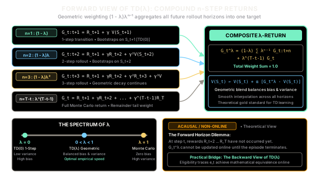
The forward view of TD(lambda) evaluates states by taking a geometrically weighted average of all n-step returns, compounding immediate and distant rollouts into a single target. By exponentially discounting distant backups, it smoothly bridges one-step temporal difference learning and complete Monte Carlo rollouts.
Why Does This Exist?
In value-based reinforcement learning, choosing how far into the future an agent should look before updating its value estimates represents a fundamental trade-off:
- One-step Temporal Difference learning [TD(0)] looks ahead exactly one transition. It enjoys low target variance and enables real-time online updates, but suffers from high bootstrapping bias because early value predictions are inherently noisy and inaccurate.
- Monte Carlo (MC) methods look ahead across the entire trajectory until termination. They have zero bootstrapping bias because they rely exclusively on realized rewards, but suffer from high target variance as stochastic state transitions and action choices compound multiplicatively over time.
- Multi-step TD (-step TD) compromises by looking ahead steps before bootstrapping. While effective, choosing a single fixed horizon is arbitrary: a 3-step return might perform best in short-horizon subgoals, while a 15-step return might excel in long corridors.
This leads to a central question: why restrict the learning target to an arbitrary single horizon ? Any convex combination of valid returns—where non-negative weights sum to one—produces a mathematically sound update target.
The forward view of solves this problem by defining the -return (). Instead of picking a single , it combines all future -step returns into a single composite target weighted by an exponential decay parameter . Shorter, low-variance horizons receive the greatest weight, while longer, low-bias horizons receive progressively decaying contributions.
Crucially, the geometric weighting is not an arbitrary artistic curve: its unique memoryless property allows this seemingly impractical, forward-looking theoretical target to be computed causally, online, and backward in time via eligibility traces—the foundation of the backward view of .
Think of It Like This
An Acoustic Echo Chamber in a Concert Hall
Imagine you sit in a concert hall listening to a violinist strike a single, resonant note:
- The direct sound (1-step return): The sound wave traveling directly from the instrument string to your ears arrives almost instantaneously. It is sharp, distinct, and carries minimal acoustic distortion—the highest immediate weight .
- The early reflections (2-step and 3-step returns): Milliseconds later, sound waves bounce off the adjacent proscenium walls and ceiling, reaching your ears with slightly reduced intensity. These reflections add body and depth without blurring the pitch—weighted by and .
- The decaying reverberation tail (distant -step and Monte Carlo returns): Sound waves that bounced off distant balconies and back walls arrive later still, their acoustic energy decaying geometrically by a constant wall absorption factor at every bounce.
- The total perception (-return): You do not hear an isolated, bone-dry pluck in an anechoic chamber (), nor do you hear an unintelligible wash of endless reflections in an echoing marble cave (). You perceive a harmonious, integrated acoustic experience that combines the crisp clarity of the initial transient with the rich context of decaying echoes.
Where the analogy breaks down: In acoustics, sound reflections travel across physical space and reach your ear forward in physical time. In reinforcement learning, the "reflections" are future rewards and state values that have not occurred yet at time step . To compute the compound echo at time in the forward view, you would have to listen to sounds that will be played minutes into the future. Furthermore, physical acoustic decay is dictated by room geometry, whereas is a deliberate algorithmic hyperparameter tuned to balance estimation bias and rollout variance.
How It Actually Works
Mathematical Formulation of the Compound -Return
To understand the forward view, we first construct the family of -step returns and then aggregate them geometrically.
1. The -Step Return Family
For a state visited at time , the -step return accumulates realized rewards for consecutive time steps and bootstraps on the estimated value of state :
where:
- is the discount factor.
- is the reward received at step .
- is the value estimate of state at step .
- If (where is the terminal time step of an episode), all remaining rewards beyond termination are zero, and the return collapses to the complete Monte Carlo return :
2. The Continuing / Infinite-Horizon -Return
In an infinite-horizon task, the forward -return is defined as the geometrically weighted sum of all -step returns for :
where . Notice that the geometric weights sum exactly to one:
Because the weights form a valid probability distribution over horizons , the -return is a true convex combination of valid return targets.
3. Episodic Truncation at Terminal Step
In episodic tasks that terminate at time step , there are only distinct transitions remaining. Every -step return for is identical to the complete Monte Carlo return :
Summing the infinite tail of geometric weights for all :
This gives the practical episodic formula for the forward -return:
The finite sum weights , and the terminal tail receives the remaining weight . Their sum is identically .
4. Boundary Cases: The Spectrum of
- When : The -return reduces strictly to the standard one-step TD(0) return.
- When : The -return reduces strictly to the full trajectory Monte Carlo return.
- When : The -return smoothly interpolates between TD(0) and Monte Carlo, allowing the agent to capture long-range consequences while retaining the variance-damping stability of bootstrapping.
5. The Forward-View Value Update
The theoretical forward-view update rule updates the value of state toward the composite target :
where is the step-size parameter.
Worked numerical example
Consider a 3-step episodic trajectory:
Let the hyperparameter values be:
- Discount factor
- Geometric blending factor
- Step size
- Terminal state value
Suppose current state value estimates before this episode are:
We evaluate the forward -return at time . Here, total episode length , so .
Step 1: Compute All Individual -Step Returns from
-
1-step return ():
-
2-step return ():
-
3-step terminal return (, Full Monte Carlo Return ):
Step 2: Compute Geometric Weight Weights
For , the weights assigned to , , and are:
- Weight for ():
- Weight for ():
- Weight for (, terminal tail):
Check total weight:
Step 3: Compute the Composite Target
Multiply each -step return by its geometric weight:
- Contribution from :
- Contribution from :
- Contribution from :
Sum the weighted components:
Step 4: Compare with the Extreme Boundaries
- Under (TD(0)): Target is .
- Under (Monte Carlo): Target is .
- Under : Target is , smoothly balancing the low 1-step target and the high full rollout return.
Step 5: Update State Value
Applying the forward-view update with step size :
The state value increases from to .
Code
Below is a self-contained, type-hinted Python script that implements the forward-view -return calculation from trajectory logs and verifies boundary convergence across the entire spectrum:
from dataclasses import dataclassfrom typing import Dict, List, Optional, Tuple
@dataclass(frozen=True)class Transition: """Represents a single experienced transition step.""" state: str reward: float next_state: str
def compute_n_step_return( trajectory: List[Transition], start_idx: int, n: int, gamma: float, values: Dict[str, float],) -> float: """Compute the n-step return G_{t:t+n} starting from trajectory[start_idx]. If start_idx + n reaches or exceeds the terminal step, bootstraps on 0.0. """ total_steps = len(trajectory) horizon = min(start_idx + n, total_steps) accumulated_return = 0.0 discount = 1.0
# Sum discounted rewards along the n-step horizon for k in range(start_idx, horizon): accumulated_return += discount * trajectory[k].reward discount *= gamma
# If the horizon did not reach terminal step T, bootstrap on V(S_{t+n}) if start_idx + n < total_steps: bootstrap_state = trajectory[start_idx + n].state accumulated_return += discount * values.get(bootstrap_state, 0.0)
return accumulated_return
def compute_forward_lambda_returns( trajectory: List[Transition], gamma: float, lam: float, values: Dict[str, float],) -> List[float]: """Compute the forward lambda-return G_t^lambda for every time step t. Uses the episodic truncation formula: G_t^lambda = (1 - lam) * sum_{n=1}^{T-t-1} lam^(n-1) * G_{t:t+n} + lam^(T-t-1) * G_t """ total_steps = len(trajectory) lambda_returns: List[float] = []
for t in range(total_steps): steps_remaining = total_steps - t # Compute all valid n-step returns for n in 1 ... steps_remaining n_step_returns = [ compute_n_step_return(trajectory, t, n, gamma, values) for n in range(1, steps_remaining + 1) ]
# Blend n-step returns with geometric weights g_lambda = 0.0 for idx in range(steps_remaining - 1): n = idx + 1 weight = (1.0 - lam) * (lam ** (n - 1)) g_lambda += weight * n_step_returns[idx]
# The terminal tail accumulates all remaining weight terminal_weight = lam ** (steps_remaining - 1) g_lambda += terminal_weight * n_step_returns[-1]
lambda_returns.append(g_lambda)
return lambda_returns
def run_forward_td_demonstration() -> None: # 3-step trajectory matching the numerical example trajectory: List[Transition] = [ Transition(state="S0", reward=2.0, next_state="S1"), Transition(state="S1", reward=1.0, next_state="S2"), Transition(state="S2", reward=4.0, next_state="ST"), ]
values: Dict[str, float] = {"S0": 1.0, "S1": 3.0, "S2": 5.0, "ST": 0.0} gamma = 0.9 lam = 0.7 alpha = 0.1
print("--- Individual n-Step Returns at t=0 ---") for n in range(1, 4): g_n = compute_n_step_return(trajectory, 0, n, gamma, values) print(f"G_0:{n} = {g_n:.4f}")
# Compute compound forward targets g_lambda_all = compute_forward_lambda_returns(trajectory, gamma, lam, values) print(f"\nG_0^lambda (lambda={lam}): {g_lambda_all[0]:.4f}") print(f"G_1^lambda (lambda={lam}): {g_lambda_all[1]:.4f}") print(f"G_2^lambda (lambda={lam}): {g_lambda_all[2]:.4f}")
print("\n--- Lambda Spectrum at t=0 ---") for test_lam in [0.0, 0.5, 0.7, 1.0]: g_val = compute_forward_lambda_returns(trajectory, gamma, test_lam, values)[0] print(f"lambda={test_lam:.1f} -> G_0^lambda = {g_val:.4f}")
# Offline Forward-View Value Updates updated_values = dict(values) for t, step in enumerate(trajectory): target = g_lambda_all[t] updated_values[step.state] += alpha * (target - updated_values[step.state])
print("\n--- Updated Values after Forward Pass ---") for s in ["S0", "S1", "S2"]: print(f"V({s}): {values[s]:.4f} -> {updated_values[s]:.4f}")
if __name__ == "__main__": run_forward_td_demonstration()
# -> Expected output:# -> --- Individual n-Step Returns at t=0 ---# -> G_0:1 = 4.7000# -> G_0:2 = 6.9500# -> G_0:3 = 6.1400# -> # -> G_0^lambda (lambda=0.7): 5.8781# -> G_1^lambda (lambda=0.7): 4.8700# -> G_2^lambda (lambda=0.7): 4.0000# -> # -> --- Lambda Spectrum at t=0 ---# -> lambda=0.0 -> G_0^lambda = 4.7000# -> lambda=0.5 -> G_0^lambda = 5.6225# -> lambda=0.7 -> G_0^lambda = 5.8781# -> lambda=1.0 -> G_0^lambda = 6.1400# -> # -> --- Updated Values after Forward Pass ---# -> V(S0): 1.0000 -> 1.4878# -> V(S1): 3.0000 -> 3.1870# -> V(S2): 5.0000 -> 4.9000Watch Out For
The Acausal Lookahead Trap: Confusing Theory with Online Execution
The forward view is mathematically elegant, but it is acausal: it looks forward into time. At time step , computing requires knowing rewards and states up to the end of the episode.
The Symptom: Practitioners attempting to implement forward directly in interactive agents encounter critical architectural failures:
- The agent cannot learn online: An interactive agent driving a robot or trading in financial markets cannot update its state value at step because future market ticks or camera frames have not happened yet.
- Failure on continuing tasks: In non-terminating tasks where , the forward target can never be finalized, causing memory buffers to grow unboundedly.
- Delayed feedback latency: Delaying all updates to the end of an episode reintroduces Monte Carlo-like latency, preventing early transitions from accelerating learning during the rollout itself.
The Fix: Understand the role of the forward view: it is a theoretical gold standard (a conceptual target), not an operational online algorithm.
- To execute online and step-by-step, use the backward view of with eligibility traces ().
- Sutton and Barto's equivalence theorem proves that under offline batch updates with linear function approximation, the sum of offline backward updates is identical to the sum of offline forward updates.
- By updating states backward in time based on how frequently and recently they were visited, eligibility traces achieve the forward view's geometric weighting causally and incrementally at computation per step.
The Quick Version
- Compound Geometric Averaging: The forward view of constructs a single composite target, the -return , by calculating a geometrically decaying average of all possible -step returns with weights .
- Unifying the Spectrum: acts as an interpolation knob between pure 1-step temporal difference learning (, low variance, high bias) and full-trajectory Monte Carlo evaluation (, zero bias, high variance).
- Exact Convex Weights: For episodic tasks, all weights beyond horizon accumulate into the full return with weight , guaranteeing that weights always sum strictly to .
- Theoretical Target vs. Online Implementation: Because the forward view requires future transitions, it cannot run causally online; it serves as the theoretical benchmark faithfully implemented by the backward view via eligibility traces.