Backward View of TD(lambda)

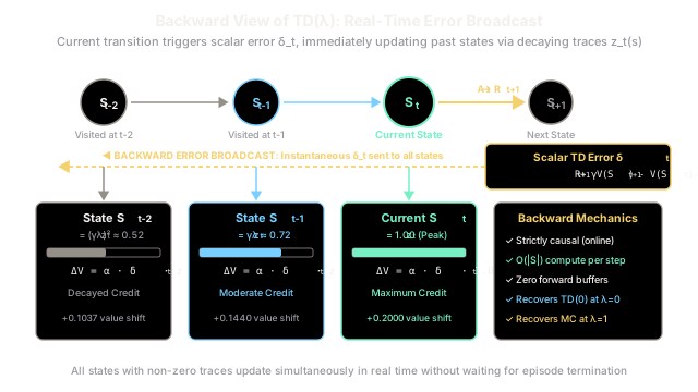
Rather than waiting for an episode to finish to assign credit, the backward view maintains a decaying memory trace of recently visited states. When a transition occurs, the resulting temporal-difference error is broadcast backward in real time, updating all recently visited states simultaneously.

Why Does This Exist?

In reinforcement learning, the theoretical formulation of temporal-difference learning with multi-step horizons—known as the forward view of $\text{TD}(\lambda)$ —is conceptually elegant. It defines the compound $\lambda$ -return $G_t^\lambda$ as a geometrically weighted average of all possible future $n$ -step returns.

However, the forward view suffers from a critical practical limitation: it is fundamentally acausal. To evaluate the $\lambda$ -return for a state visited at time $t$ , the agent must look ahead into future time steps until the episode concludes. In continuing tasks that never terminate, or in physical real-time applications such as robotics and high-frequency control, an agent cannot halt execution to wait for the distant future before learning.

Storing full trajectory buffers also imposes substantial memory overhead and delays credit assignment. If an agent takes an action that precipitates a reward ten steps later, waiting ten steps or until episode completion prevents the agent from making immediate course corrections.

The backward view of $\text{TD}(\lambda)$ exists to transform this theoretical forward-looking concept into an online, causal, and incremental mechanism. Instead of looking forward into unobserved future steps, the agent looks backward at a fading memory record of recently visited states. Whenever an unexpected transition or reward occurs, the agent calculates a single scalar Temporal Difference error $\delta_t$ and broadcasts it backward across all states in memory. Each state absorbs an update proportional to its current eligibility trace.

This allows $\text{TD}(\lambda)$ to execute in real time at every discrete time step $t$ with $O(|\mathcal{S}|)$ memory and compute, without storing trajectory histories.

Think of It Like This

The Megaphone on the Mountain Trail

Imagine a group of runners navigating a winding mountain trail with numbered checkpoints: checkpoint $A$ , then checkpoint $B$ , and finally checkpoint $C$ .

As the runners progress along the trail, a trail marshal stationed at checkpoint $C$ suddenly spots an unexpected boulder blocking the path ahead (a surprise negative event) or discovers an unmapped fresh water spring (a surprise positive reward).

Instead of writing a letter and waiting for runners to finish the race hours later, the marshal immediately blasts an alert over a high-powered megaphone: "Surprise condition discovered at mile 3!"

The sound wave radiates backward across the entire trail:

The runner who just stepped past checkpoint $C$ one second ago hears the horn at maximum, piercing volume ( $z = 1.0$ ) and immediately alters their pace.
The runner who passed checkpoint $B$ two minutes ago hears a moderately loud echo ( $z = 0.72$ ) and adjusts their pacing moderately.
The runner who passed checkpoint $A$ five minutes ago hears only a faint, muffled rumble in the distance ( $z = 0.52$ ) and makes a minor note.
Runners resting back at the starting lodge who haven't set foot on the trail hear nothing at all ( $z = 0.0$ ).

In this scenario:

The marshal's blast is the scalar TD error $\delta_t$ : an instantaneous measurement of surprise at the current location.
The acoustic volume heard by each runner is their eligibility trace $z_t(s)$ : a fading physical memory of how recently and frequently they occupied that sector of the trail.
Every active runner adapts their strategy simultaneously the moment the horn sounds, without anyone waiting for the race to finish.

Where the analogy stops: Sound waves dissipate in physical air due to geometric dispersion and terrain obstacles. In reinforcement learning, eligibility trace decay is an exact mathematical exponential factor ( $\gamma \lambda$ ) governed strictly by the algorithm's hyperparameters.

How It Actually Works

Mechanistic Online Formulation: Scalar Error and Eligibility Traces

The backward view of $\text{TD}(\lambda)$ operates as an incremental, causal filter over discrete states and transitions.

At each time step $t$ , the agent maintains two tables over the state space $\mathcal{S}$ :

Value function estimates: $V_t \in \mathbb{R}^{|\mathcal{S}|}$ , where entry $V_t(s)$ represents the expected cumulative return from state $s$ .
Eligibility trace vector: $z_t \in \mathbb{R}^{|\mathcal{S}|}$ , where entry $z_t(s)$ tracks how eligible state $s$ is for receiving credit from current prediction errors.

At the start of an episode, all eligibility traces are initialized to zero:

z_{-1}(s) = 0 \quad \forall s \in \mathcal{S}

When the agent transitions from state $S_t$ to state $S_{t+1}$ after taking action $A_t$ and observing reward $R_{t+1}$ , the algorithm executes three operations:

1. Trace Decay and Accumulation

The agent updates the eligibility trace of every state in the environment. Under the standard accumulating traces formulation:

z_t(s) = \begin{cases} \gamma \lambda z_{t-1}(s) + 1 & \text{if } s = S_t \\ \gamma \lambda z_{t-1}(s) & \text{if } s \neq S_t \end{cases}

Using the indicator function $\mathbf{1}(s = S_t)$ , this is expressed concisely as:

z_t(s) = \gamma \lambda z_{t-1}(s) + \mathbf{1}(s = S_t) \quad \forall s \in \mathcal{S}

where:

$\gamma \in [0, 1]$ is the discount factor.
$\lambda \in [0, 1]$ is the trace-decay parameter governing memory retention.
The product $\gamma \lambda \in [0, 1]$ represents the per-step decay multiplier applied to all dormant traces.
The visited state $S_t$ receives an immediate eligibility boost of $+1$ .

(Note: Under replacing traces, the visited state is set directly to $z_t(S_t) = 1$ rather than incremented by $1$ , which prevents trace values from exceeding unity in frequently revisited states).

2. Compute Scalar TD Error

The agent calculates the one-step Temporal Difference error $\delta_t$ generated by the current transition:

\delta_t = R_{t+1} + \gamma V_t(S_{t+1}) - V_t(S_t)

where $V_t(S_{t+1}) = 0$ if $S_{t+1}$ is a terminal absorbing state.

Crucially, $\delta_t$ is a single scalar that quantifies the local discrepancy between the observed transition and the agent's prior prediction.

3. Error Broadcast and Parallel Value Updates

Rather than updating only the current state $S_t$ , the scalar error $\delta_t$ is broadcast across all states in memory:

V_{t+1}(s) = V_t(s) + \alpha \delta_t z_t(s) \quad \forall s \in \mathcal{S}

where $\alpha \in (0, 1]$ is the step-size learning rate parameter.

A state visited on the current step ( $z_t(s) \approx 1$ ) receives the full weight of the update: $\alpha \delta_t$ .
A state visited several steps ago ( $0 < z_t(s) < 1$ ) receives a decayed fraction of the update: $\alpha \delta_t z_t(s)$ .
A state that has not been visited during the episode ( $z_t(s) = 0$ ) receives zero update.

Complexity and Equivalence

Memory Complexity: $O(|\mathcal{S}|)$ to store the trace array $z$ alongside the value array $V$ .
Computational Complexity: $O(|\mathcal{S}|)$ operations per time step. In practice, this can be reduced to $O(|\text{active states}|)$ by maintaining a sparse set of states with $z_t(s) > \epsilon$ .
Theoretical Equivalence: In episodic tasks with offline or infinitesimal step-size updates, the total cumulative value change accumulated across an episode under the backward view matches the theoretical forward-view $\lambda$ -return exactly: $\sum_{t=0}^{T-1} \Delta V_t^{\text{backward}}(s) = \sum_{t=0}^{T-1} \alpha \left[ G_t^\lambda - V(S_t) \right] \mathbf{1}(S_t = s)$

Worked numerical calculation

Consider an agent navigating a 3-state chain environment that terminates after state $C$ :

A \xrightarrow{R_1 = 0.0} B \xrightarrow{R_2 = 1.0} C \xrightarrow{R_3 = 5.0} \text{Terminal}

We set the parameters:

Discount factor: $\gamma = 0.9$
Trace decay parameter: $\lambda = 0.8$
Decay rate: $\gamma \lambda = 0.9 \times 0.8 = 0.72$
Learning rate: $\alpha = 0.1$

The initial tabular values are:

$V_0(A) = 1.0000$
$V_0(B) = 2.0000$
$V_0(C) = 3.0000$
$V_0(\text{Terminal}) = 0.0000$

All traces begin at zero: $z_{-1}(A) = z_{-1}(B) = z_{-1}(C) = 0.0000$ .

Step 0: Transition $A \to B$ with Reward $R_1 = 0.0$

Update Traces: $z_0(A) = 0.72 \times 0.0 + 1.0 = 1.0000, \quad z_0(B) = 0.0000, \quad z_0(C) = 0.0000$
Compute TD Error: $\delta_0 = R_1 + \gamma V_0(B) - V_0(A) = 0.0 + 0.9(2.0000) - 1.0000 = 1.8000 - 1.0000 = +0.8000$
Update Values ( $V_1(s) = V_0(s) + 0.1 \times \delta_0 \times z_0(s)$ ):
- $V_1(A) = 1.0000 + 0.1(0.8000)(1.0000) = 1.0000 + 0.0800 = \mathbf{1.0800}$
- $V_1(B) = 2.0000 + 0.1(0.8000)(0.0000) = \mathbf{2.0000}$
- $V_1(C) = 3.0000 + 0.1(0.8000)(0.0000) = \mathbf{3.0000}$

Step 1: Transition $B \to C$ with Reward $R_2 = 1.0$

Update Traces (Trace for $A$ decays; trace for $B$ accumulates): $\begin{aligned} z_1(A) &= 0.72 \times z_0(A) = 0.72 \times 1.0000 = \mathbf{0.7200} \\ z_1(B) &= 0.72 \times z_0(B) + 1.0 = 0.72 \times 0.0 + 1.0 = \mathbf{1.0000} \\ z_1(C) &= 0.72 \times 0.0 = \mathbf{0.0000} \end{aligned}$
Compute TD Error: $\delta_1 = R_2 + \gamma V_1(C) - V_1(B) = 1.0 + 0.9(3.0000) - 2.0000 = 1.0 + 2.7000 - 2.0000 = +1.7000$
Update Values ( $V_2(s) = V_1(s) + 0.1 \times \delta_1 \times z_1(s)$ ):
- $V_2(A) = 1.0800 + 0.1(1.7000)(0.7200) = 1.0800 + 0.1224 = \mathbf{1.2024}$
- $V_2(B) = 2.0000 + 0.1(1.7000)(1.0000) = 2.0000 + 0.1700 = \mathbf{2.1700}$
- $V_2(C) = 3.0000 + 0.1(1.7000)(0.0000) = \mathbf{3.0000}$

Notice that state $A$ receives a $+0.1224$ credit update during step 1 even though the agent was transitioning between $B$ and $C$ !

Step 2: Transition $C \to \text{Terminal}$ with Reward $R_3 = 5.0$

Update Traces (All past traces decay by 0.72; $C$ accumulates): $\begin{aligned} z_2(A) &= 0.72 \times z_1(A) = 0.72 \times 0.7200 = \mathbf{0.5184} \\ z_2(B) &= 0.72 \times z_1(B) = 0.72 \times 1.0000 = \mathbf{0.7200} \\ z_2(C) &= 0.72 \times z_1(C) + 1.0 = 0.72 \times 0.0 + 1.0 = \mathbf{1.0000} \end{aligned}$
Compute TD Error: $\delta_2 = R_3 + \gamma V_2(\text{Terminal}) - V_2(C) = 5.0 + 0.9(0.0) - 3.0000 = 5.0000 - 3.0000 = +2.0000$
Update Values ( $V_3(s) = V_2(s) + 0.1 \times \delta_2 \times z_2(s)$ ):
- $V_3(A) = 1.2024 + 0.1(2.0000)(0.5184) = 1.2024 + 0.1037 = \mathbf{1.3061}$
- $V_3(B) = 2.1700 + 0.1(2.0000)(0.7200) = 2.1700 + 0.1440 = \mathbf{2.3140}$
- $V_3(C) = 3.0000 + 0.1(2.0000)(1.0000) = 3.0000 + 0.2000 = \mathbf{3.2000}$

At the terminal transition, the large positive reward ( $+5.0$ ) creates a scalar surprise of $\delta_2 = +2.0000$ , which immediately flows back to update $C$ , $B$ , and $A$ simultaneously in a single broadcast pass.

Code

1from typing import Dict, List, Optional, Tuple2
3
4class BackwardViewTDLambda:5    """Tabular Backward View TD(lambda) state-value predictor with accumulating traces."""6
7    def __init__(8        self,9        states: List[str],10        gamma: float = 0.9,11        lam: float = 0.8,12        alpha: float = 0.1,13        initial_values: Optional[Dict[str, float]] = None,14    ) -> None:15        """Initialize value tables and eligibility traces.16
17        Args:18            states: List of discrete state identifiers.19            gamma: Discount factor in [0, 1].20            lam: Trace-decay parameter lambda in [0, 1].21            alpha: Learning rate parameter in (0, 1].22            initial_values: Optional initial state values dictionary.23        """24        self.states = states25        self.gamma = gamma26        self.lam = lam27        self.alpha = alpha28        self.values: Dict[str, float] = (29            initial_values.copy() if initial_values else {s: 0.0 for s in states}30        )31        # Eligibility trace vector z in R^{|S|} initialized to zero32        self.traces: Dict[str, float] = {s: 0.0 for s in states}33
34    def reset_traces(self) -> None:35        """Reset all eligibility traces to zero at the start of an episode."""36        for s in self.states:37            self.traces[s] = 0.038
39    def step_update(40        self,41        current_state: str,42        reward: float,43        next_state: str,44        done: bool,45    ) -> Tuple[float, Dict[str, float], Dict[str, float]]:46        """Perform a single-step online backward-view TD(lambda) update.47
48        Args:49            current_state: State S_t visited at time step t.50            reward: Scalar reward R_{t+1} received upon transition.51            next_state: State S_{t+1} reached after transition.52            done: Boolean flag indicating if next_state is terminal.53
54        Returns:55            Tuple of (td_error, snapshot_of_traces, snapshot_of_updated_values).56        """57        # 1. Update eligibility traces for all states (accumulating traces)58        # z_t(s) = gamma * lambda * z_{t-1}(s) + 1(s == S_t)59        decay = self.gamma * self.lam60        for s in self.states:61            self.traces[s] = decay * self.traces[s] + (1.0 if s == current_state else 0.0)62
63        # 2. Compute local TD error: delta_t = R_{t+1} + gamma * V(S_{t+1}) - V(S_t)64        v_next = 0.0 if done else self.values[next_state]65        v_curr = self.values[current_state]66        delta_t = reward + self.gamma * v_next - v_curr67
68        # 3. Broadcast TD error to update all states in memory:69        # V_{t+1}(s) = V_t(s) + alpha * delta_t * z_t(s)70        for s in self.states:71            self.values[s] += self.alpha * delta_t * self.traces[s]72
73        return delta_t, self.traces.copy(), self.values.copy()74
75
76# Execution and automated verification matching the worked numerical walk77agent = BackwardViewTDLambda(78    states=["A", "B", "C"],79    gamma=0.9,80    lam=0.8,81    alpha=0.1,82    initial_values={"A": 1.0, "B": 2.0, "C": 3.0},83)84
85# Step 0: Transition A -> B, Reward = 0.086d0, z0, v0 = agent.step_update(87    current_state="A", reward=0.0, next_state="B", done=False88)89assert abs(d0 - 0.8000) < 1e-490assert abs(z0["A"] - 1.0000) < 1e-491assert abs(v0["A"] - 1.0800) < 1e-492print(f"Step 0 (A->B) | delta: {d0:.4f} | V(A): {v0['A']:.4f}")93
94# Step 1: Transition B -> C, Reward = 1.095d1, z1, v1 = agent.step_update(96    current_state="B", reward=1.0, next_state="C", done=False97)98assert abs(d1 - 1.7000) < 1e-499assert abs(z1["A"] - 0.7200) < 1e-4100assert abs(z1["B"] - 1.0000) < 1e-4101assert abs(v1["A"] - 1.2024) < 1e-4102assert abs(v1["B"] - 2.1700) < 1e-4103print(f"Step 1 (B->C) | delta: {d1:.4f} | V(A): {v1['A']:.4f} | V(B): {v1['B']:.4f}")104
105# Step 2: Transition C -> Terminal, Reward = 5.0106d2, z2, v2 = agent.step_update(107    current_state="C", reward=5.0, next_state="Terminal", done=True108)109assert abs(d2 - 2.0000) < 1e-4110assert abs(z2["A"] - 0.5184) < 1e-4111assert abs(z2["B"] - 0.7200) < 1e-4112assert abs(z2["C"] - 1.0000) < 1e-4113assert abs(v2["A"] - 1.3061) < 1e-4114assert abs(v2["B"] - 2.3140) < 1e-4115assert abs(v2["C"] - 3.2000) < 1e-4116print(f"Step 2 (C->End)| delta: {d2:.4f} | V(A): {v2['A']:.4f} | V(B): {v2['B']:.4f} | V(C): {v2['C']:.4f}")117
118# -> Step 0 (A->B) | delta: 0.8000 | V(A): 1.0800119# -> Step 1 (B->C) | delta: 1.7000 | V(A): 1.2024 | V(B): 2.1700120# -> Step 2 (C->End)| delta: 2.0000 | V(A): 1.3061 | V(B): 2.3140 | V(C): 3.2000

Watch Out For

Failing to Decay Traces on Zero-Reward Steps or Across Episode Boundaries

A pervasive implementation error occurs when developers only decay or update eligibility traces when a non-zero reward is received, or forget to reset traces at episode boundaries.

The Failure Mode:

Conditional Decay Bug: Writing if reward != 0: decay_traces() halts trace decay during long zero-reward corridors. Unvisited states maintain stale, inflated eligibility traces. When a reward is finally encountered, ancient states absorb massive, unearned value shifts, causing value estimates to diverge.
Episode Bleed Bug: Forgetting to call reset_traces() when an agent reaches a terminal state and begins a new episode leaves non-zero traces active. Early actions in episode 2 receive credit for rewards encountered late in episode 1, corrupting credit assignment across independent trials.

Concrete Fix:

Always apply the decay factor $\gamma \lambda$ unconditionally at every single transition $t$ , regardless of whether $R_{t+1} = 0$ : $z_t(s) \leftarrow \gamma \lambda z_{t-1}(s) \quad \forall s \neq S_t$
Explicitly zero out the trace vector $z$ $z$ inside the environment's reset() callback at every episode boundary:
```
1def start_new_episode(self):2    for s in self.states:3        self.traces[s] = 0.0
```
In environments with long recurring loops, evaluate replacing traces ( $z_t(S_t) \leftarrow 1$ ) rather than accumulating traces ( $z_t(S_t) \leftarrow z_t(S_t) + 1$ ) to prevent trace magnitude from compounding unboundedly when a state is frequently visited within a short window.

The Quick Version

The backward view of $\text{TD}(\lambda)$ provides a causal, online mechanism that updates value functions in real time without waiting for future rewards or episode termination.
An eligibility trace vector $z_t(s)$ acts as a decaying memory filter, decaying by $\gamma \lambda$ each time step and boosting visited states by $+1$ .
Each transition computes an instantaneous scalar TD error $\delta_t = R_{t+1} + \gamma V(S_{t+1}) - V(S_t)$ , which is broadcast backward to update all states in memory via $\Delta V(s) = \alpha \delta_t z_t(s)$ .
At episode termination, the cumulative updates of the backward view match the theoretical forward-view $\lambda$ -return while maintaining an $O(|\mathcal{S}|)$ memory and compute footprint.