Evolution Strategies (ES)

Evolution strategies tune a policy without backpropagation: they shake the weights with Gaussian noise, score each shaky copy, and step toward the noise that scored best.

Evolution strategies score Gaussian perturbations of the policy weights in parallel and step toward the perturbations with the highest returns.

Why Does This Exist?

Most policy optimization leans on gradients. You run stochastic gradient descent in RL, which needs a differentiable loss, backpropagation through the policy, and careful handling of moving bootstrap targets. That machinery breaks down when the policy is not differentiable (a simulator with discrete switches, a programmatic controller), when rewards arrive only at the end of a long episode, or when you have thousands of CPUs and a gradient method that cannot keep them all fed.

Evolution strategies (ES), in the form Salimans et al. described in 2017 ("Evolution Strategies as a Scalable Alternative to Reinforcement Learning"), take a different deal. Forget derivatives entirely: treat the whole environment as a black box that maps a weight vector to one number, the episode return. Shake the weights with Gaussian noise, run one episode per shaky copy, and move the weights toward the noise that scored well. Each episode is independent, so the work splits across as many parallel workers as you own, and workers exchange only random seeds plus scalar returns instead of gradients or weight vectors.

This page covers the Gaussian-perturbation estimator, the two variance tricks that make it practical (antithetic sampling and rank shaping), and why it scales. For the gradient-based counterpart, read policy gradient methods. For how ES keeps searching instead of collapsing early, see exploration vs. exploitation.

Think of It Like This

The Foggy-Hill Scout Team

You are camped on a foggy hill and want the summit, but you cannot see more than a few steps. Each morning you send out four scouts, each walking a short fixed distance in a random compass direction, then shouting back their altitude. You move camp a small step toward the average of the scouts' directions, weighted by how high each one got.

The mapping is exact: your camp is the weight vector $\theta$ , each scout's walk is a perturbation $\sigma \epsilon$ , the shouted altitude is the episode return $F$ , and the camp move is the update. You also send scouts in opposite pairs (one northeast, one southwest), so a slope that lifts one and drops the other tells you the direction twice as clearly: that is antithetic sampling. And if one scout stumbles onto a helicopter pad with a silly altitude reading, you rank the reports instead of trusting raw numbers: that is fitness shaping.

Where the analogy stops: your hill has two or three directions, while a policy has thousands of weights, so ES needs far more scouts than four. Real scouts also report exact altitudes, while episode returns are noisy, which is why the step size stays small and the noise scale $\sigma$ needs tuning.

How It Actually Works

Write $\theta$ for the policy weights (a flat vector with $d$ entries), $F(\theta)$ for the total episode return earned by running the policy with those weights, $\sigma$ for the noise scale (a small positive number), and $\epsilon$ for one perturbation drawn from a standard Gaussian, $\epsilon \sim \mathcal{N}(0, I)$ . Smoothing the return with noise gives $J(\theta) = \mathbb{E}[F(\theta + \sigma \epsilon)]$ , whose gradient has a form you can sample without any derivative:

$g = \frac{1}{n \sigma} \sum_{i=1}^{n} F(\theta + \sigma \epsilon_i) \, \epsilon_i$

Each term pushes $\theta$ along $\epsilon_i$ in proportion to the return that perturbation earned. Then $\theta \leftarrow \theta + \alpha g$ , with $\alpha$ the step size. That is the whole optimizer: perturb, score, step.

Why antithetic sampling halves the variance

Instead of $n$ independent perturbations, ES draws $m$ of them and evaluates both signs, $\theta + \sigma \epsilon_i$ and $\theta - \sigma \epsilon_i$ . The estimator becomes:

$g = \frac{1}{2 m \sigma} \sum_{i=1}^{m} \big(F(\theta + \sigma \epsilon_i) - F(\theta - \sigma \epsilon_i)\big) \, \epsilon_i$

The difference cancels any baseline shift shared by the pair, so a region where every return is uniformly high or low contributes no noise. You get $2m$ episode scores for $m$ random draws, and each pair votes on its axis with the contrast between its two ends.

Why rank shaping tames wild returns

Raw returns are badly behaved: one lucky episode can outscore everything else combined, and adding a constant to all rewards should change nothing but would rescale the step. So in practice $F$ is replaced by a shaped utility $u$ computed from ranks. Sort the $2m$ scores, map the best to a positive utility and the worst to a negative one (centered so the utilities sum to zero), and use $u$ in place of $F$ . The update then depends only on ordering, never on reward scale, offsets, or outliers.

Why it scales to thousands of workers

Episodes never interact, so worker $k$ can score its own perturbations alone. The Salimans design goes one step further with a shared noise table: every worker holds the same pre-generated Gaussian table and indexes into it with a seed, so workers broadcast only (seed, scalar return) pairs. Communication per episode stays tiny while the population grows into the thousands, which is how ES rivalled then-standard policy-gradient methods on locomotion and game benchmarks despite using no gradients at all. The price is sample hunger: ES typically needs far more episodes than a gradient method to reach the same policy, so you only pay it when gradients are unavailable or parallelism is nearly free.

Worked numerical example

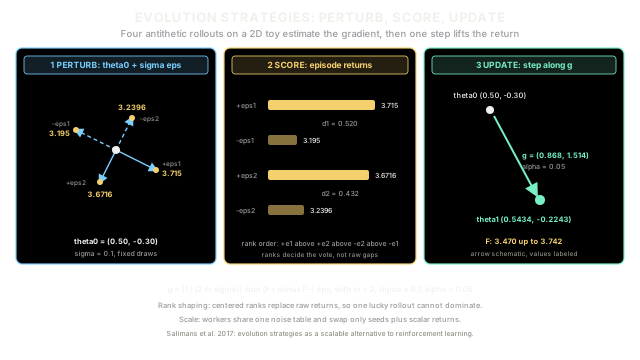
Take a 2D toy with return $F(\theta) = -(\theta_1 - 1)^2 - 2(\theta_2 - 0.5)^2 + 5$ , best at $[1.0, 0.5]$ with value $5.0$ . Start at $\theta_0 = [0.5, -0.3]$ (return $3.470$ ), set $\sigma = 0.1$ and step size $\alpha = 0.05$ , and fix two perturbation draws $\epsilon_1 = [1.0, 0.5]$ and $\epsilon_2 = [-0.4, 0.8]$ .

Score the four antithetic copies:

$\theta_0 + 0.1 \, \epsilon_1 = [0.6, -0.25]$ , return $3.715$
$\theta_0 - 0.1 \, \epsilon_1 = [0.4, -0.35]$ , return $3.195$
$\theta_0 + 0.1 \, \epsilon_2 = [0.46, -0.22]$ , return $3.6716$
$\theta_0 - 0.1 \, \epsilon_2 = [0.54, -0.38]$ , return $3.2396$

Pair contrasts: $d_1 = 3.715 - 3.195 = 0.520$ and $d_2 = 3.6716 - 3.2396 = 0.432$ . The gradient estimate with $m = 2$ pairs is:

$g = \frac{1}{2 \times 2 \times 0.1} \big(0.520 \, \epsilon_1 + 0.432 \, \epsilon_2\big) = 2.5 \times [0.3472, 0.6056] = [0.868, 1.514]$

Step once: $\theta_1 = [0.5, -0.3] + 0.05 \times [0.868, 1.514] = [0.5434, -0.2243]$ . The new return is $3.742$ , up from $3.470$ . Notice the estimate points the same way as the true gradient $[1.0, 3.2]$ (both entries positive) but with sampling noise on the magnitudes: that is the ES bargain in miniature. With only ranks kept, the ordering $F_1^+ > F_2^+ > F_2^- > F_1^-$ alone would drive the same directional vote.

Code

A pure-Python transcription of the worked example above. It scores the four antithetic copies, forms the estimate, and takes one step.

1def toy_return(theta: list[float]) -> float:2    """Quadratic toy return. Best at [1.0, 0.5], where it equals 5.0."""3    return -((theta[0] - 1.0) ** 2) - 2.0 * ((theta[1] - 0.5) ** 2) + 5.04
5
6def es_step(7    theta: list[float],8    perturbations: list[list[float]],9    sigma: float,10    step_size: float,11) -> tuple[list[float], list[float]]:12    """One antithetic ES update: score +sigma*e and -sigma*e, then step."""13    pairs = [14        (15            toy_return([theta[0] + sigma * e[0], theta[1] + sigma * e[1]]),16            toy_return([theta[0] - sigma * e[0], theta[1] - sigma * e[1]]),17        )18        for e in perturbations19    ]20    gradient = [21        sum((plus - minus) * e[i] for (plus, minus), e in zip(pairs, perturbations))22        / (2.0 * len(perturbations) * sigma)23        for i in range(2)24    ]25    updated = [theta[i] + step_size * gradient[i] for i in range(2)]26    return updated, gradient27
28
29theta0 = [0.5, -0.3]30new_theta, grad = es_step(theta0, [[1.0, 0.5], [-0.4, 0.8]], sigma=0.1, step_size=0.05)31print([round(v, 3) for v in grad])       # -> [0.868, 1.514]32print([round(v, 4) for v in new_theta])  # -> [0.5434, -0.2243]33print(round(toy_return(theta0), 3), round(toy_return(new_theta), 3))  # -> 3.47 3.742

Watch Out For

Sigma set without looking at the return gap

The noise scale $\sigma$ decides whether the $\pm$ pair carries any signal. Too large, and the perturbations land in unrelated parts of the landscape: returns swing wildly, the estimate is mostly noise, and the policy thrashes instead of climbing. Too small, and $F(\theta + \sigma \epsilon)$ and $F(\theta - \sigma \epsilon)$ differ by less than the episode-to-episode noise, so the update chases randomness and learning stalls while looking busy.

The fix: scale $\sigma$ to your weights (a starting point near a hundredth to a tenth of the typical weight magnitude), then watch one diagnostic, the average $|F^+ - F^-|$ over pairs. If the gap is indistinguishable from the noise you see when repeating the exact same weights twice, raise $\sigma$ . If single perturbations change returns by a large fraction of the total return range, lower it.

Unreproducible runs from unshared noise

ES runs are only reproducible if you can replay the exact perturbations. The classic failure: each worker samples its own noise from an unseeded generator, the run improves, and nobody can reconstruct which $\epsilon$ produced the winning update, so the result cannot be audited or debugged. A subtler variant logs the returns but not the seeds.

The fix, borrowed from the original large-scale design: generate one shared noise table up front, hand workers (seed index, return) pairs, and log the table seed plus $\sigma$ and $\alpha$ with every experiment. Then any single perturbation is exactly replayable from its index, and a rerun with the same table seed reproduces the whole optimization path.

The Quick Version

Evolution strategies optimize a policy with no derivatives: they score Gaussian perturbations of the weights and step toward the noise that earned the best returns.
The antithetic estimator scores $\theta + \sigma \epsilon$ and $\theta - \sigma \epsilon$ per draw, so shared baseline shifts cancel and each pair votes with its contrast.
Rank shaping replaces raw returns with centered rank utilities, making the update immune to reward scale, offsets, and one lucky outlier episode.
Workers share a noise table and exchange only seeds plus scalar returns, which lets ES use thousands of parallel CPUs with tiny communication.
The trade is sample hunger: ES needs far more episodes than gradient methods, so reach for it when the policy is non-differentiable or parallelism is nearly free.