Evolutionary Methods and Neuroevolution

Instead of computing gradients, keep a population of policies, score each one, and breed the winners with small random tweaks until behavior improves.

A population of four policies is scored, the top two are selected as parents, and crossover plus mutation builds the next generation without any gradient.

Why Does This Exist?

Gradients need a slope to follow. In reinforcement learning that slope often does not exist. The reward can be sparse, like a game that pays only after hundreds of correct moves. It can be deceptive, where the nearby improvement points away from the real goal. Or the policy itself can be non-differentiable, like a discrete rule set, a compiled simulator, or a physical robot you cannot backpropagate through.

Policy gradient methods handle continuous actions by estimating a gradient from returns, and deep reinforcement learning adds neural networks that learn features from raw input. Both still assume you can nudge parameters in the direction of higher return and get a useful signal. When the reward stays flat for long stretches, that nudge carries no information and learning stalls. That flat reward search is the same problem behind exploration versus exploitation: you must try far-apart behaviors before you can refine any of them.

Evolution takes a different deal. Do not compute a derivative at all. Keep a population of full policies, run each one, score it with episode return, keep the winners, mix them, add random tweaks, and repeat. It works with any reward function and any policy form because it only looks at scores, never at slopes.

This page teaches that shared umbrella loop: selection, crossover, and mutation, plus when to reach for it. It also sketches the three specialized children so you can tell them apart: Evolution Strategies, which samples Gaussian noise around a mean policy; CMA-ES, which adapts the shape of that sampling distribution as it learns; and NEAT, which grows both network weights and network topology starting from small nets with speciation to protect new ideas. Those three have no dedicated pages in this change, so they get summaries here and no links.

Think of It Like This

Saving seeds from your best tomato plants

You plant four tomato varieties in spring. At harvest you taste each row and weigh the yield. You save seeds only from the two tastiest, most productive rows. Next spring you plant those saved seeds, cross two of the best plants to mix traits, and accept that a little natural variation will show up on its own. You also replant your single best row unchanged, in case the new mixes flop.

The map is direct. The four rows are the population. Taste plus yield is fitness, the episode return. Saving only two rows is truncation selection. Mixing two plants is crossover. Natural variation is mutation. Replanting the best row unchanged is elitism.

Where the analogy stops: your garden gives you one harvest per year with weather noise you cannot control. Here you choose the fitness function, usually total episode return, and you choose the tweak size, usually a Gaussian spread you can shrink over time. You also test every candidate from the same start, which no garden lets you do.

How It Actually Works

Call the policy weights $\theta$ . That is one flat vector holding every number the policy needs, whether it is four scalars or four million network weights. Call fitness $f(\theta)$ . That is the score you get after running the policy, usually total episode return. Call $N$ the population size, here $N = 4$ . Call $k$ the number of survivors you breed from, here $k = 2$ . Call $\sigma$ the mutation spread, here $\sigma = 0.1$ , the standard deviation of the Gaussian noise you add.

One generation runs five steps:

Start with $N$ weight vectors.
Evaluate each one for one or more full episodes and record $f$ .
Select the top $k$ scorers and discard the rest.
Vary the survivors by crossover, often a plain average, plus mutation, usually fresh samples from $\mathcal{N}(0, \sigma^2)$ added to each weight.
Replace the old population with the children, keeping the single best parent unchanged, and repeat.

No gradient appears anywhere. The only signal is the ranking of scores.

Three flavors you will meet

Evolution Strategies keeps a mean vector $m$ and samples children as $m + \sigma \epsilon$ with $\epsilon$ drawn from a standard Gaussian. It then moves $m$ toward the noise directions that scored well. OpenAI popularized this form for RL because shared random seeds let thousands of workers generate the same perturbations without sending big weight vectors around.

CMA-ES keeps the same sampling idea but also learns the covariance $C$ of the noise, so sampling becomes $m + \sigma \mathcal{N}(0, C)$ . When one direction keeps paying off, the distribution stretches along it. That helps on stretched, ill-conditioned problems where a round ball wastes samples, at the price of more bookkeeping per step.

NEAT evolves the network itself, not just its weights. It starts from small nets with no hidden units, adds nodes and links by mutation, tracks every new gene with a historical marking so two nets can be crossed over sensibly, and groups similar topologies into species that share fitness so a promising new shape is not killed before its weights catch up.

Worked example: selecting from four policies

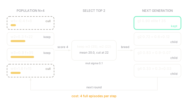
Take four one-weight policies with these measured returns:

$w_1 = -0.4$ , $f_1 = 8$
$w_2 = 0.3$ , $f_2 = 22$
$w_3 = 0.9$ , $f_3 = 35$
$w_4 = 1.6$ , $f_4 = 15$

Total fitness is $8 + 22 + 35 + 15 = 80$ . Mean fitness is $80 / 4 = 20.0$ . Ranked best to worst: $w_3$ at 35, $w_2$ at 22, $w_4$ at 15, $w_1$ at 8. Truncation with $k = 2$ keeps $w_3$ and $w_2$ and drops the rest. The cut sits at 22, so anything below 22 is gone.

Crossover averages the two parents:

$(0.9 + 0.3) / 2 = 1.2 / 2 = 0.6$

Now apply the fixed mutation draws for teaching, all consistent with $\sigma = 0.1$ :

Crossover child: $0.6 + 0.12 = 0.72$
Copy of best parent: $0.9 - 0.07 = 0.83$
Copy of second parent: $0.3 + 0.03 = 0.33$

With elitism the next generation is:

$g_1 = 0.90$ , elite copy of $w_3$ , fitness 35 carried
$g_2 = 0.72$ , crossover plus mutation
$g_3 = 0.83$ , best parent mutated
$g_4 = 0.33$ , second parent mutated

Those four weights cluster near the two winners, 0.3 and 0.9, which is exactly what you want after one step. None of the children has a score yet. The next step must run four fresh episodes to score them, which is why the diagram closes the loop back to the population and flags the cost at the bottom.

Code

1from typing import List, Tuple2
3weights: List[float] = [-0.4, 0.3, 0.9, 1.6]4fitness: List[float] = [8.0, 22.0, 35.0, 15.0]5
6mean_f: float = sum(fitness) / len(fitness)7ranked: List[Tuple[float, float]] = sorted(8    zip(weights, fitness), key=lambda t: t[1], reverse=True9)10parents: List[Tuple[float, float]] = ranked[:2]11child_mean: float = round((parents[0][0] + parents[1][0]) / 2.0, 2)12
13elite: float = parents[0][0]14child_crossover: float = round(child_mean + 0.12, 2)15child_best: float = round(parents[0][0] - 0.07, 2)16child_second: float = round(parents[1][0] + 0.03, 2)17next_gen: List[float] = [elite, child_crossover, child_best, child_second]18
19print(f"mean fitness: {mean_f:.1f}")20print(f"parents: {parents}")21print(f"child mean: {child_mean:.2f}")22print(f"next gen: [{elite:.2f}, {child_crossover:.2f}, {child_best:.2f}, {child_second:.2f}]")

1# -> expected output:2mean fitness: 20.03parents: [(0.9, 35.0), (0.3, 22.0)]4child mean: 0.605next gen: [0.90, 0.72, 0.83, 0.33]

Watch Out For

Sample inefficiency: each step burns full episodes

The symptom is slow wall-clock progress. This page used 4 episodes for one update. Real runs use hundreds or thousands of policies per generation, and each one needs full episodes before the update. If your simulator is slow or each episode runs minutes on hardware, one generation can take all day.

The fix is to match the tool to the reward. When rewards are dense and the policy is differentiable, prefer policy gradient methods because each episode gives gradient information for every step. When you must evolve, parallelize rollouts across workers, share random seeds instead of weight vectors, and start with small populations before scaling up.

Premature convergence: everyone crowds the first winner

The symptom is a population that looks done after a few rounds but scores poorly. All weights sit near 0.9 in the example, variation shrinks toward zero, and no child ever tries far regions again. Greedy top-k selection plus tiny sigma causes this fast.

The fix is to protect diversity on purpose. Raise sigma early and shrink it later, use tournament selection instead of always taking the top two, keep an elite of one rather than half the population, and restart or inject fresh random members when the spread of fitness drops near zero for several rounds.

The Quick Version

Neuroevolution scores whole policies and breeds winners, so it works without differentiable losses or slope signals.
One generation selects the top scorers, mixes parents by averaging, then adds Gaussian noise with spread sigma.
The four-policy example scores 8, 22, 35 and 15 for mean 20.0 and keeps the policies at 0.9 and 0.3.
Crossover mean 0.6 plus fixed tweaks builds the next generation at 0.90, 0.72, 0.83 and 0.33 before rescoring.
Evolution fits sparse, deceptive, or non-differentiable rewards; gradients fit dense rewards with cheap differentiable policies.