Value Decomposition Networks (VDN)

Why Does This Exist?

In cooperative Multi-Agent RL, a team of $N$ agents must collaborate in a shared environment to maximize a single scalar team reward $r(s, \mathbf{a})$. Before Value Decomposition Networks (VDN), practitioners faced two equally unappealing architectural extremes:

1. Independent Q-Learning (IQL): Each agent trains its own independent Q-network $Q_i(s_i, a_i)$, treating all teammates as part of the passive environment. Because all agents learn simultaneously, the environment appears non-stationary. More critically, IQL suffers from spurious credit assignment and the lazy agent problem: when a team receives a reward, an agent that contributed nothing (or made a mistake) receives positive reinforcement simply because a teammate carried the objective. Conversely, an agent making an optimal move gets penalized if a teammate blunders.
2. Centralized Q-Learning: A single master network evaluates the entire joint action-value function $Q(s, a_1, a_2, \dots, a_N)$. While mathematically sound, this approach suffers from an exponential combinatorial explosion: the joint action space scales as $|\mathcal{A}|^N$. For 8 agents with 5 discrete actions each, evaluating greedy actions requires searching over $5^8 = 390{,}625$ action combinations at every step. Furthermore, centralized execution requires instant, zero-latency communication across all agents during physical deployment—an impossible requirement in decentralized swarms or radio-denied robotics.

Introduced by Sunehag et al. in 2017, Value Decomposition Networks (VDN) resolve this impasse through Centralized Training with Decentralized Execution (CTDE). VDN hypothesizes that the joint team value function can be modeled as the linear sum of individual agent utility functions: $Q_{\text{tot}} = \sum_{i=1}^N Q_i$. By exploiting the mathematical properties of additive factorization, VDN satisfies the Individual-Global-Max (IGM) property: maximizing the global team value is strictly equivalent to each agent greedily maximizing its own local utility. This allows agents to train centrally against team rewards while executing completely independently without communication.

Think of It Like This

How It Actually Works

The Cooperative Credit Assignment Dilemma

Consider a fully cooperative stochastic game defined on a shared state $s \in \mathcal{S}$ with $N$ agents. At each timestep $t$, each agent $i$ observes a private local observation $o_i \in \mathcal{O}_i$ drawn from observation function $O(s, i)$. Because agents have partial observability, each agent maintains an action-observation history:

The agents concurrently execute joint action $\mathbf{a} = (a_1, \dots, a_N) \in \mathcal{A}^N$, transitioning the environment to $s'$ and generating a single shared scalar team reward $r(s, \mathbf{a})$.

The fundamental objective is to learn individual policies $\pi_i(a_i | \tau_i)$ that maximize the team's discounted cumulative return:

In a decentralized system, agent $i$ must choose action $a_i$ conditioned only on its private history $\tau_i$, without knowing the simultaneous actions $\mathbf{a}_{-i}$ chosen by teammates.

Additive Factorization and the IGM Property

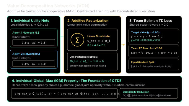
VDN resolves this decentralized execution challenge by introducing the additive value factorization architecture:

1[Agent 1 History tau_1] ---> [Agent 1 Network Q_1(tau_1, a_1)] ---\2                                                                     \3[Agent 2 History tau_2] ---> [Agent 2 Network Q_2(tau_2, a_2)] ----> [ + ] ---> Q_tot(tau, a)4                                                                     /             |5[Agent N History tau_N] ---> [Agent N Network Q_N(tau_N, a_N)] ---/               v6                                                                        [Team Bellman Loss L(theta)]7                                                                        Target y = r + gamma * max Q_tot'

1. Additive Factorization

VDN represents the joint action-value function $Q_{\text{tot}}(\boldsymbol{\tau}, \mathbf{a})$ as the linear summation of individual agent utilities:

where each $Q_i$ is parameterized by a deep neural network (typically a Recurrent Neural Network or GRU to handle partially observable histories $\tau_i$).

2. The Individual-Global-Max (IGM) Property

Because addition is strictly monotonic with respect to each component ($\frac{\partial Q_{\text{tot}}}{\partial Q_i} = 1 > 0$), the joint argmax operator distributes cleanly across individual utility functions:

This identity is the core of Centralized Training with Decentralized Execution (CTDE):

• During Centralized Training: The full joint network $Q_{\text{tot}}$ is evaluated and trained using global replay data.
• During Decentralized Execution: Each agent $i$ simply chooses its action greedily using its own local network: $$a_i^* = \arg\max_{a_i} Q_i(\tau_i, a_i)$$ No communication channels or knowledge of co-players' utilities are required during runtime.

3. Efficient Bellman Target Computation

In centralized Q-learning, evaluating the target value requires searching over the combinatorial joint action space: $\max_{\mathbf{a}'} Q(s', \mathbf{a}')$ which requires $\mathcal{O}(|\mathcal{A}|^N)$ operations.

Under VDN's additive factorization, the maximization distributes inside the sum:

This reduces the target search complexity from exponential $\mathcal{O}(|\mathcal{A}|^N)$ to linear $\mathcal{O}(N \cdot |\mathcal{A}_i|)$, unlocking scalable training for large multi-agent teams.

4. Training Loss and Gradient Distribution

The entire architecture is trained end-to-end by minimizing the standard DQN mean-squared Bellman error:

Because the mixing function is a direct sum, the gradient with respect to each agent's utility is:

The temporal difference error $\delta = y - Q_{\text{tot}}$ is distributed symmetrically and equally to all agent sub-networks.

Worked numerical example

Let us trace a concrete learning step on a 2-agent cooperative task ($\mathcal{A}_1 = \{A, B\}$, $\mathcal{A}_2 = \{A, B\}$, discount $\gamma = 0.90$):

Step 1: Local Utility Evaluation At local history $\boldsymbol{\tau} = (\tau_1, \tau_2)$, the individual networks output utility values:

• Agent 1: $$Q_1(\tau_1, A) = 3.50, \quad Q_1(\tau_1, B) = 1.00 \implies a_1^* = \arg\max(3.50, 1.00) = A$$
• Agent 2: $$Q_2(\tau_2, A) = 2.50, \quad Q_2(\tau_2, B) = 4.00 \implies a_2^* = \arg\max(2.50, 4.00) = B$$

Both agents independently execute joint action $\mathbf{a} = (A, B)$ without communication.

Step 2: Additive Total Joint Value Evaluation The joint total Q-value is the linear sum:

Step 3: Environment Interaction The team executes $(A, B)$ in the environment, transitioning to next history $\boldsymbol{\tau}'$ and receiving a shared scalar team reward:

Step 4: Compute Target Utilities at $\boldsymbol{\tau}'$ The target networks (with parameters $\theta^-$) evaluate local utilities for the next state:

• Agent 1 target net: $$Q_1'(\tau_1', A) = 4.00, \quad Q_1'(\tau_1', B) = 2.00 \implies \max_{a_1'} Q_1' = 4.00$$
• Agent 2 target net: $$Q_2'(\tau_2', A) = 3.00, \quad Q_2'(\tau_2', B) = 5.00 \implies \max_{a_2'} Q_2' = 5.00$$

Step 5: Centralized Bellman Target Evaluation Using the distributed IGM property:

The target value is:

Step 6: TD Error and Gradient Splitting The team temporal difference error is:

The squared Bellman loss is:

During backward propagation:

The positive prediction error ($\delta = +2.60$) pushes both agent utilities upward symmetrically by an equal unit gradient.

Code

1import numpy as np2
3
4class ValueDecompositionNetwork:5    """Simulates Value Decomposition Networks (VDN) for cooperative MARL:6
7    Additive value factorization, Individual-Global-Max (IGM) property,8    centralized Bellman target computation, and symmetric TD gradient splitting.9    """10
11    def __init__(self, gamma: float = 0.90) -> None:12        self.gamma = gamma13
14    def compute_joint_q_tot(self, utilities: list[float]) -> float:15        """Additively factorizes joint Q_tot = sum_i Q_i."""16        return float(np.sum(utilities))17
18    def select_decentralized_actions(19        self, q_tables: list[dict[str, float]]20    ) -> list[str]:21        """Each agent independently selects its action via local greedy argmax:22
23        a_i* = argmax_{a_i} Q_i(tau_i, a_i). Satisfies IGM without communication.24        """25        return [max(q_tab, key=q_tab.get) for q_tab in q_tables]26
27    def compute_bellman_target(28        self, reward: float, next_q_tables: list[dict[str, float]]29    ) -> float:30        """Computes centralized team Bellman target in O(N * |A|) time:31
32        y = r + gamma * sum_i max_{a'_i} Q_i'(tau'_i, a'_i)33        """34        max_next_sum = sum(max(q_tab.values()) for q_tab in next_q_tables)35        target = reward + self.gamma * max_next_sum36        return float(target)37
38    def compute_td_error_and_loss(39        self, q_tot: float, target: float40    ) -> tuple[float, float, float, float]:41        """Computes Bellman TD error, MSE loss, and unit gradient splits."""42        td_error = target - q_tot43        loss = 0.5 * (td_error**2)44        grad_q1 = 1.0 * td_error45        grad_q2 = 1.0 * td_error46        return float(td_error), float(loss), float(grad_q1), float(grad_q2)47
48
49if __name__ == "__main__":50    np.set_printoptions(precision=4, suppress=True)51
52    vdn = ValueDecompositionNetwork(gamma=0.90)53
54    # Utilities from the worked numerical example55    q1_current = {"A": 3.5, "B": 1.0}56    q2_current = {"A": 2.5, "B": 4.0}57
58    # Step 1: Decentralized action selection (IGM)59    actions = vdn.select_decentralized_actions([q1_current, q2_current])60    chosen_utilities = [q1_current[actions[0]], q2_current[actions[1]]]61
62    # Step 2: Joint Q_tot evaluation63    q_tot = vdn.compute_joint_q_tot(chosen_utilities)64
65    # Step 3: Next state utilities and Bellman target66    q1_next = {"A": 4.0, "B": 2.0}67    q2_next = {"A": 3.0, "B": 5.0}68    reward = 2.069    target = vdn.compute_bellman_target(reward, [q1_next, q2_next])70
71    # Step 4: TD error and loss72    td_error, loss, g1, g2 = vdn.compute_td_error_and_loss(q_tot, target)73
74    print(f"Decentralized Actions Chosen: a1={actions[0]}, a2={actions[1]}")75    # -> Decentralized Actions Chosen: a1=A, a2=B76
77    print(f"Joint Q_tot(tau, (A, B)): {q_tot:.2f}")78    # -> Joint Q_tot(tau, (A, B)): 7.5079
80    print(f"Centralized Bellman Target y: {target:.2f}")81    # -> Centralized Bellman Target y: 10.1082
83    print(f"TD Error delta: {td_error:.2f}")84    # -> TD Error delta: 2.6085
86    print(f"Squared Bellman Loss: {loss:.2f}")87    # -> Squared Bellman Loss: 3.3888
89    print(90        f"Symmetric Gradient Splitting: dL/dQ1 = {g1:.2f}, dL/dQ2 = {g2:.2f}"91    )92    # -> Symmetric Gradient Splitting: dL/dQ1 = 2.60, dL/dQ2 = 2.6093
94    # Assert correctness against theoretical values95    assert actions == ["A", "B"]96    assert np.isclose(q_tot, 7.50, atol=1e-2)97    assert np.isclose(target, 10.10, atol=1e-2)98    assert np.isclose(td_error, 2.60, atol=1e-2)99    assert np.isclose(loss, 3.38, atol=1e-2)100    assert np.isclose(g1, 2.60, atol=1e-2)101    assert np.isclose(g2, 2.60, atol=1e-2)

Watch Out For

The Quick Version

• Additive Factorization: VDN resolves the cooperative multi-agent credit assignment problem by decomposing the team value function into the sum of local utilities: $Q_{\text{tot}}(\boldsymbol{\tau}, \mathbf{a}) = \sum_i Q_i(\tau_i, a_i)$.
• Individual-Global-Max (IGM): Because summation is strictly monotonic, each agent can greedily pick $a_i^* = \arg\max_{a_i} Q_i(\tau_i, a_i)$ locally during deployment without any inter-agent communication.
• Linear Target Complexity: Reduces Bellman target maximization from combinatorial $\mathcal{O}(|\mathcal{A}|^N)$ to linear $\mathcal{O}(N \cdot |\mathcal{A}|)$ by distributing the $\max$ operator inside the sum.
• Structural Limitation: VDN cannot represent non-monotonic value matrices where optimal actions depend non-linearly on teammates' choices, directly motivating advanced architectures like QMIX and QTRAN.

What to Read Next

• QMIX and QTRAN
• Multi-Agent PPO (MAPPO)
• Multi-Agent DDPG (MADDPG)