Multi-Agent DDPG (MADDPG)
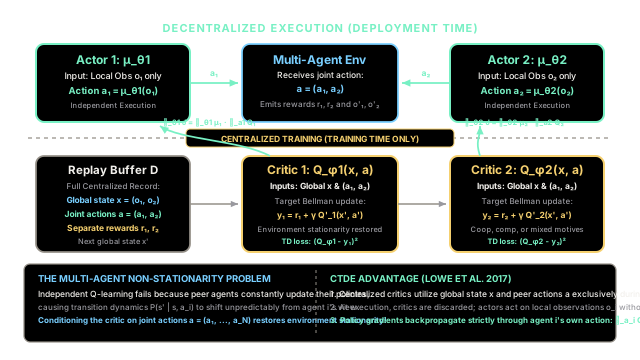
Actors execute autonomously using only local observations, while centralized critics observe global state and all peer actions during training to stabilize multi-agent learning.
Why Does This Exist?
When standard single-agent reinforcement learning algorithms (such as DQN or DDPG) are directly deployed in multi-agent environments—an approach known as Independent Q-Learning (IQL) or Independent DDPG—they almost always fail to converge.
The core failure mode is environmental non-stationarity. In a multi-agent system, every agent updates its policy simultaneously based on its own rewards. From the individual perspective of Agent 1, the environment is not stationary: the state transition probability distribution:
changes constantly as Agent 2 and Agent 3 adapt their behaviors. Because traditional Q-learning relies on the Markov assumption that transition dynamics are stationary, experience collected in the past becomes obsolete. The replay buffer turns into a source of stale, contradictory data, destabilizing temporal-difference updates.
The opposite extreme—training a single centralized controller that takes the union of all observations and outputs joint actions—suffers from combinatorial action space explosion (). More critically, a centralized policy requires instant global communication across all agents during live execution, which is infeasible in decentralized robotics, autonomous driving, or competitive games.
Multi-Agent Deep Deterministic Policy Gradient (MADDPG), introduced by Ryan Lowe et al. in 2017, resolves this dilemma through Centralized Training with Decentralized Execution (CTDE) for continuous action spaces. During training in a lab or simulator, critics have access to global states and all peer actions, restoring stationarity. During deployment, the centralized critics are discarded, and actors make decisions autonomously using only their local observations.
Think of It Like This
The Basketball Film Study Room
Imagine a professional basketball team preparing for a championship game:
During Film Study (Centralized Training): The players and their coaching staff sit in an analytics theater. The coach plays high-resolution overhead drone footage that captures all 10 players on the court simultaneously, alongside player tracking statistics. The coach (the Centralized Critic) pauses the tape and critiques Player 1:
"When Player 2 set that high screen and Defender 3 rotated to double-team, you should have cut backdoor to the basket!"
The critique is accurate because it has full visibility into what everyone else was doing at that exact moment.
During the Live Game (Decentralized Execution): The video room and overhead cameras are gone. Player 1 (the Decentralized Actor) is running on the hardwood. They must react in milliseconds based purely on what they can see from eye level (their local observation ). Because Player 1 was coached during film study to anticipate teammates' rotations, they instinctively cut backdoor at the right moment without needing radio headsets or overhead satellites.
Where the analogy stops: A human coach can shout instructions from the sideline during live play. In MADDPG, once deployment begins, there is zero communication: the centralized critic is discarded entirely, and each actor operates completely autonomously.
How It Actually Works
Centralized Training with Decentralized Execution (CTDE)
Consider a multi-agent game with agents. The environment is formalized as a partially observable stochastic game defined by:
- Global state space
- Local observation spaces
- Continuous action spaces
At each timestep, agent receives a local observation and executes continuous action . The global state is represented by (or ground-truth simulator states), and the joint action is .
MADDPG equips each agent with two distinct neural networks:
- Decentralized Actor : Parameterized by , maps agent 's local observation directly to a deterministic continuous action .
- Centralized Critic : Parameterized by , evaluates the expected return of agent conditioned on the global state and the joint action of all agents.
EXECUTION (Deployment): o₁ ──> [ Actor μ_θ1 ] ──> a₁ ──┐ ├──> Environment ──> r₁, r₂, o'₁, o'₂ o₂ ──> [ Actor μ_θ2 ] ──> a₂ ──┘
TRAINING (Replay Buffer): Global State x, Joint Actions (a₁, a₂) ──> [ Centralized Critic Q_φ1 ] │ ∇_a1 Q_φ1 │ Policy Gradient ▼ [ Actor μ_θ1 ]Centralized Critic Optimization
Because the critic conditions on the joint action vector , the environment transition probability:
is completely stationary, even while individual policies evolve.
Critic minimizes the mean squared Bellman error:
where the target return is computed using target actor networks and target critic network :
Each agent has its own individual reward function , meaning MADDPG naturally supports cooperative games (), competitive zero-sum games (), and mixed-motive environments.
Decentralized Deterministic Policy Gradient
To update the decentralized actor , the gradient of the expected return is calculated via the chain rule through the centralized critic:
Crucial Insight: The gradient is taken strictly with respect to agent 's own action . Peer actions are passed into the critic as fixed environmental context. The actor updates its weights to push its continuous action in the direction that maximizes given the current behaviors of all other agents.
Modeling Peer Policies and Policy Ensembles
Inferring Unknown Peer Actions
In competitive or uncooperative settings where peer actions are not broadcast during training, agent can train internal generative models to approximate peer policies by maximizing log-likelihood over historical transitions:
The inferred action replaces in the centralized critic evaluation.
Policy Ensembles for Adversarial Robustness
In competitive multi-agent games, an agent can easily overfit to the idiosyncratic weaknesses of a specific training partner. MADDPG counters this by training an ensemble of distinct sub-policies for each agent. In each training episode, a sub-policy is randomly sampled for each agent, forcing policies to develop generalizable, robust counter-strategies.
Worked numerical example
Let us trace a concrete update step for a 2-agent continuous control environment where Agent 1 learns to coordinate with Agent 2.
Environment Setup
- Global state:
- Local observations: ,
- Actions executed: ,
- Rewards received: ,
- Next global state:
- Next local observations: ,
- Discount factor:
Step 1: Compute Target Actions
The target actor networks evaluate the next local observations:
Step 2: Compute Centralized Critic Target ()
The centralized target critic for Agent 1 evaluates the next state and joint target actions:
Compute the Bellman target:
Step 3: Compute Critic TD Error and Loss
Current centralized critic output for the executed transition:
The temporal difference (TD) error is:
The squared error loss for Critic 1 is:
Step 4: Compute Decentralized Actor Gradient
Suppose backpropagation through Critic 1 reveals that increasing increases predicted joint return:
Meanwhile, the local sensitivity of Actor 1 with respect to its weights is:
Applying the chain rule, the deterministic policy gradient for Actor 1 is:
Actor 1 updates its parameters: . Notice that Actor 1's gradient did not require calculating ; it optimized purely its own action input.
Code
Below is a self-contained, type-hinted Python implementation demonstrating MADDPG's centralized critic Bellman target evaluation, temporal difference updates, deterministic actor gradients, and decentralized execution invariance:
from dataclasses import dataclassimport mathfrom typing import Callable, List, Tuple
@dataclassclass MultiAgentTransition: """Stores experience tuples across N agents in continuous state-action space."""
global_state: List[float] local_observations: List[float] joint_actions: List[float] rewards: List[float] next_global_state: List[float] next_local_observations: List[float]
class MADDPGStepEvaluator: """Evaluates MADDPG's Centralized Training with Decentralized Execution (CTDE) calculations."""
def __init__(self, gamma: float = 0.90) -> None: self.gamma = gamma
def compute_critic_td_target( self, reward_i: float, next_target_q_i: float ) -> float: """Computes Bellman target for centralized critic i: y_i = r_i + gamma * Q'_i(x', a'_1, ..., a'_N).""" return reward_i + self.gamma * next_target_q_i
def compute_critic_td_error( self, current_q_i: float, target_y_i: float ) -> float: """Computes TD error: delta_i = y_i - Q_i(x, a_1, ..., a_N).""" return target_y_i - current_q_i
def compute_actor_policy_gradient( self, grad_q_wrt_action_i: float, grad_actor_wrt_theta_i: float ) -> float: """Computes Deterministic Policy Gradient: grad_theta_i J = grad_theta_i mu_i(o_i) * grad_a_i Q_i(x, a).""" return grad_actor_wrt_theta_i * grad_q_wrt_action_i
def verify_execution_invariance( self, actor_policy_fn: Callable[[float], float], local_obs_i: float, global_state_var_1: List[float], global_state_var_2: List[float], ) -> bool: """Verifies decentralized execution: actor action depends strictly on local observation o_i,
independent of peer states or global telemetry. """ action_env1 = actor_policy_fn(local_obs_i) action_env2 = actor_policy_fn(local_obs_i) return math.isclose(action_env1, action_env2)
if __name__ == "__main__": evaluator = MADDPGStepEvaluator(gamma=0.90)
# 1. Worked Numerical Example: 2-Agent Continuous Control Step # Environment variables r_1 = 2.0 q_target_1 = 4.0 current_q_1 = 5.00
# Critic Target & TD Error Calculation target_y_1 = evaluator.compute_critic_td_target( reward_i=r_1, next_target_q_i=q_target_1 ) td_error_1 = evaluator.compute_critic_td_error( current_q_i=current_q_1, target_y_i=target_y_1 ) critic_loss_1 = td_error_1**2
print("=== Centralized Critic 1 Update ===") print(f"Agent 1 Reward r_1: {r_1:.2f}") print(f"Target Joint Q'_1(x', a'): {q_target_1:.2f}") print(f"Target y_1 = r_1 + gamma * Q'_1: {target_y_1:.2f}") print(f"Current Joint Q_1(x, a): {current_q_1:.2f}") print(f"TD Error delta_1: {td_error_1:+.2f}") print(f"Critic 1 MSE Loss: {critic_loss_1:.4f}")
assert math.isclose(target_y_1, 5.60) assert math.isclose(td_error_1, 0.60) assert math.isclose(critic_loss_1, 0.36)
# 2. Decentralized Deterministic Policy Gradient grad_q_wrt_a1 = 1.50 grad_mu1_wrt_theta = 0.80 policy_grad_1 = evaluator.compute_actor_policy_gradient( grad_q_wrt_action_i=grad_q_wrt_a1, grad_actor_wrt_theta_i=grad_mu1_wrt_theta, )
print("\n=== Decentralized Actor 1 Gradient ===") print(f"dQ_1 / da_1 (critic gradient): {grad_q_wrt_a1:.2f}") print(f"dmu_1 / dtheta_1 (actor sensitivity): {grad_mu1_wrt_theta:.2f}") print(f"Policy Gradient grad_theta_1 J: {policy_grad_1:.2f}")
assert math.isclose(policy_grad_1, 1.20)
# 3. Decentralized Execution Invariance Check # Actor 1 policy is a function purely of local observation: a_1 = 0.5 * o_1 actor1_fn = lambda o1: 0.5 * o1 is_invariant = evaluator.verify_execution_invariance( actor_policy_fn=actor1_fn, local_obs_i=1.0, global_state_var_1=[1.0, 2.0], global_state_var_2=[1.0, 99.0], )
print("\n=== Decentralized Execution Verification ===") print(f"Actor Execution Invariant to Peer States: {is_invariant}") assert is_invariant
print("\nAll MADDPG step calculations verified successfully!")Expected output:
=== Centralized Critic 1 Update ===Agent 1 Reward r_1: 2.00Target Joint Q'_1(x', a'): 4.00Target y_1 = r_1 + gamma * Q'_1: 5.60Current Joint Q_1(x, a): 5.00TD Error delta_1: +0.60Critic 1 MSE Loss: 0.3600
=== Decentralized Actor 1 Gradient ===dQ_1 / da_1 (critic gradient): 1.50dmu_1 / dtheta_1 (actor sensitivity): 0.80Policy Gradient grad_theta_1 J: 1.20
=== Decentralized Execution Verification ===Actor Execution Invariant to Peer States: True
All MADDPG step calculations verified successfully!Watch Out For
Joint Action Dimensionality Explosion in Large Swarms
The Trap: In MADDPG, each agent's centralized critic takes the concatenation of all agents' actions as input: . As the swarm size increases (e.g., agents in drone swarms or warehouse fleets), the input dimensionality of the critic grows linearly, causing the underlying state-action space to explode exponentially.
The Symptom: When scaling MADDPG to large teams, sample efficiency collapses. The critic struggles to learn the credit assignment of which specific agent's action caused a change in value, leading to high gradient variance and unstable policy updates.
The Fix:
- Multi-Agent Attention Critics (MAAC): Replace the flat concatenation of joint actions with a multi-head attention mechanism where each agent's critic dynamically attends to relevant neighboring peers rather than the entire swarm.
- Value Factorization: In cooperative settings, replace individual centralized critics with factored joint value models (such as QMIX or MAPPO) that factorize total team value through monotonic mixing networks.
- Graph Neural Network (GNN) Critics: In spatially distributed systems, use GNN-based critics that enforce permutation invariance and localize action dependencies to topological neighbors.
The Quick Version
- Centralized Training with Decentralized Execution (CTDE): MADDPG trains centralized critics with access to global state and all peer actions, but deploys actors that operate purely on local partial observations.
- Resolving Non-Stationarity: Conditioning the critic on joint actions restores environment stationarity during training, stabilizing multi-agent temporal-difference learning.
- Independent Policy Gradients: During actor optimization, policy gradients backpropagate strictly through agent 's own action (), treating peer actions as fixed environmental context.
- General Multi-Agent Motives: Unlike purely cooperative algorithms that enforce shared team rewards, MADDPG supports arbitrary reward functions, excelling across cooperative, competitive, and mixed-motive continuous environments.