Information-Theoretic Regret Bounds

Why Does This Exist?

Tabular theory counts states. Its regret bounds grow with the number of state action pairs, which is fine for a gridworld and hopeless for Go, a robot arm, or anything with continuous observations. Once you approximate, states share strength through one parameterized function, as value function approximation teaches. But that raises the real question: with a function class doing the generalizing, what number now governs how long exploration takes?

Parameter count is the wrong answer. A huge network can be easy to explore when it generalizes cleanly, and a tiny class of spiky functions can force you to probe nearly everything. The linear case is solved: linear methods show the answer is the feature dimension $d$, because $d$ independent probes pin down every direction. This page lifts that idea to general classes with two related counters: eluder dimension for the bandit and online regression view, and Bellman rank for multi step RL.

Two basics before the mechanism. First, regret is the gap between the best you could have done and what you actually collected. In multi-armed bandits with arm means $\mu_a$ and best mean $\mu^*$, after $T$ pulls of arms $a_1, \dots, a_T$:

$\mathrm{Regret}(T) = \sum_{t=1}^{T} (\mu^* - \mu_{a_t})$

In RL the same idea sums $V^* - V^{\pi_t}$ over episodes, where $V^*$ is the optimal value and $V^{\pi_t}$ is the value of the policy you ran. Sublinear regret means your average mistake shrinks toward zero. Second, the tension underneath is the exploration versus exploitation dilemma: every probe that teaches you something costs reward now. These two measures tell you how many costly probes the worst case demands.

Think of It Like This

How It Actually Works

What regret counts

Read $\mathrm{Regret}(T)$ as tuition paid for learning. Each round you either pull a well understood arm (cheap, little learned) or probe something uncertain (costly now, informative). An optimistic algorithm always acts according to the most favorable world still consistent with the data, so it only suffers large regret on rounds where the probe genuinely surprises it. The whole game of these bounds is counting how many such surprises the function class admits.

Eluder dimension: counting surprises

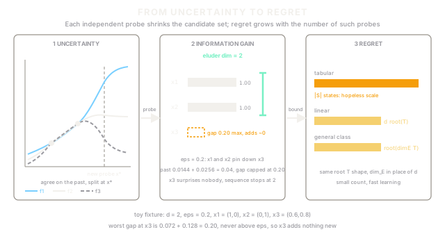
Fix a function class $\mathcal{F}$ of candidate maps from inputs $x$ (think state action pairs) to values, and a tolerance $\epsilon > 0$ (your survey tolerance: disagreements smaller than this do not matter). A new input $x_t$ is $\epsilon$ independent of past inputs $x_1, \dots, x_{t-1}$ when two functions $f, f'$ in the class agree on the whole past yet disagree now:

$\sum_{i < t} (f(x_i) - f'(x_i))^2 \le \epsilon^2 \quad \text{but} \quad |f(x_t) - f'(x_t)| > \epsilon$

The eluder dimension $\dim_E(\mathcal{F}, \epsilon)$ is the length of the longest sequence in which every input is $\epsilon$ independent of all inputs before it. Plain version: the longest run of "you could not have seen it coming" queries the class allows. Optimistic methods pay large regret only on those steps, which is why general regret bounds grow with the square root of eluder dimension times horizon, up to a log factor for the size of the class.

Worked toy: a 2D linear class has eluder dimension 2

Take $\mathcal{F} = \{x \mapsto \theta^T x\}$ with $\theta$ in $\mathbb{R}^2$ (a plane through the origin, dimension $d = 2$), tolerance $\epsilon = 0.2$, and inputs $x_1 = (1, 0)$, $x_2 = (0, 1)$, $x_3 = (0.6, 0.8)$.

First, $x_1$ is independent of the empty past: the zero function and $f(x) = \theta^T x$ with $\theta = (1, 0)$ agree vacuously on nothing observed, yet differ by $1.00 > 0.2$ at $x_1$.

Next, $x_2$ is independent of $\{x_1\}$: with $\theta = (0, 1)$ versus zero, both give $0$ at $x_1$ (past disagreement $0 \le 0.04$), yet differ by $1.00 > 0.2$ at $x_2$.

Now $x_3$ is pinned. Write $d = \theta - \theta'$ for any pair. Agreement on the past means $d_1^2 + d_2^2 \le 0.04$. The gap at $x_3$ is $0.6\, d_1 + 0.8\, d_2$, and Cauchy Schwarz caps it:

$|0.6\, d_1 + 0.8\, d_2| \le \sqrt{0.36 + 0.64} \cdot \sqrt{d_1^2 + d_2^2} = 1 \cdot 0.2 = 0.20$

never strictly above $\epsilon$. The worst case attains it exactly at $d = (0.12, 0.16)$: past disagreement $0.0144 + 0.0256 = 0.0400$, gap $0.072 + 0.128 = 0.200$. So no pair in the class surprises you at $x_3$, the longest surprising sequence has length 2, and $\dim_E = 2 = d$. The general fact behind the toy: a $d$ dimensional linear class on the unit ball has eluder dimension close to $d$, up to a $\log(1/\epsilon)$ factor.

The linear to general lift

Linear bandits run LinUCB style methods with regret shaped like $d \sqrt{T}$: dimension times root horizon. The eluder view replaces $d$ with $\dim_E(\mathcal{F}, \epsilon)$, giving regret shaped like $\sqrt{\dim_E \cdot T \cdot \log N}$, where $N$ measures how many distinct functions the class holds (a covering number). A nonlinear class with small eluder dimension inherits linear style guarantees without being linear. When someone reports that a bound "recovers LinUCB," this substitution is what they mean.

Bellman rank: the multi step version

RL adds two wrinkles bandits dodge: errors compound over horizon $H$, and the data distribution shifts as your policy changes. Bellman rank counts surprises in Bellman error space instead of raw prediction space. For a candidate value function $f$ rolled in under some policy $\pi'$, write $\mathcal{E}_h(f, \pi')$ for its average Bellman error at step $h$ (how badly $f$ violates one step consistency where $\pi'$ actually goes). The class has Bellman rank $M$ when these errors factor through $M$ dimensional vectors:

$\mathcal{E}_h(f, \pi') \approx \langle \phi_h(\pi'), \psi_h(f) \rangle$

so only $M$ independent policy versus value directions matter. Algorithms in the OLIVE family explore those directions, and their sample complexity grows polynomially in $M$ and $H$ rather than in state count. It is eluder style thinking aimed at one step inconsistencies instead of point predictions.

Code

A short check of the toy: it confirms $x_3$ is pinned at $\epsilon = 0.2$ by computing the Cauchy Schwarz cap and the equality case.

1"""Verify the 2D eluder toy: x3 is pinned by x1, x2 at eps = 0.2."""2
3import math4
5EPS = 0.26X3 = (0.6, 0.8)7
8
9def max_gap(x: tuple, eps: float) -> float:10    """Largest |x . d| with d1^2 + d2^2 <= eps^2 (Cauchy-Schwarz cap)."""11    norm_x = math.sqrt(x[0] ** 2 + x[1] ** 2)12    return norm_x * eps13
14
15def equality_case(x: tuple, eps: float) -> tuple:16    """The d attaining the cap: d = eps * x / ||x||."""17    norm_x = math.sqrt(x[0] ** 2 + x[1] ** 2)18    return (eps * x[0] / norm_x, eps * x[1] / norm_x)19
20
21bound = max_gap(X3, EPS)22d = equality_case(X3, EPS)23past = d[0] ** 2 + d[1] ** 224gap = X3[0] * d[0] + X3[1] * d[1]25
26print(f"bound at x3: {bound:.4f}")27print(f"equality d: ({d[0]:.2f}, {d[1]:.2f})")28print(f"past disagreement: {past:.4f} (eps^2 = {EPS ** 2:.4f})")29print(f"gap at x3: {gap:.4f}")30print(f"x3 independent at eps={EPS}: {gap > EPS + 1e-9}")

1# -> expected output:2bound at x3: 0.20003equality d: (0.12, 0.16)4past disagreement: 0.0400 (eps^2 = 0.0400)5gap at x3: 0.20006x3 independent at eps=0.2: False

Watch Out For

The Quick Version

• Eluder dimension is the longest run of queries that can each surprise you given all previous ones, and it sets the exploration budget for a function class.
• Optimistic methods pay large regret only on independent steps, so regret grows with the square root of eluder dimension times horizon.
• Linear classes have eluder dimension near $d$, which makes the familiar $d\sqrt{T}$ bound a special case of the general picture.
• Bellman rank applies the same counting to multi step Bellman errors, giving sample efficient RL when average errors factor through few directions.
• Neither number measures compute: small statistical complexity can still hide brutal optimization.

What to Read Next

• Multi-Armed Bandits
• Value Function Approximation
• Exploration vs. Exploitation
• Linear Methods in RL