Linear Methods in RL

Linear methods compute value estimates as a simple weighted sum of handcrafted features, guaranteeing that the mathematical error surface is a clean bowl with a single global optimum.

Linear methods compute value estimates as an inner product of weights and features, creating a convex error surface with a unique global optimum.

Why Does This Exist?

In realistic reinforcement learning applications—such as robotics, game playing, and resource allocation—the state space $\mathcal{S}$ is vast or continuous. Tabular representations, where a separate memory cell is allocated for every single state $s$ , collapse under memory limitations and fail completely to generalize: experiencing state $s$ tells a tabular agent nothing about a virtually identical state $s'$ .

To generalize across states, practitioners use function approximation. However, complex non-linear function approximators like deep neural networks introduce thorny theoretical and practical headaches: non-convex loss landscapes, local minima, saddle points, sensitivity to hyperparameter tuning, and catastrophic divergence when paired with bootstrapping and off-policy sampling (the notorious "deadly triad").

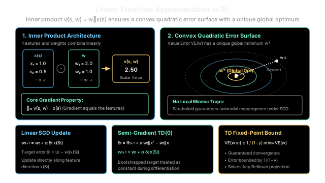
Linear methods represent the premier, theoretically sound workhorse of function approximation. By parameterizing the value function strictly as an inner product of a learnable weight vector and a feature vector, linear methods transform the value-error objective into a strictly convex quadratic bowl. There are no local minima traps, gradients compute in $O(d)$ time, and on-policy TD algorithms are mathematically guaranteed to converge to a bounded global fixed point.

Think of It Like This

The Weighted Grading Rubric

Imagine a university professor calculating a student's final course score using a syllabus rubric:

The Feature Vector $\mathbf{x}(s)$ : The student's raw performance across different categories:
- Homework assignments completed: $x_1 = 0.95$
- Midterm exam score: $x_2 = 0.82$
- Final exam score: $x_3 = 0.88$
- Class attendance: $x_4 = 1.00$
The Weight Vector $\mathbf{w}$ : The syllabus percentage allocated to each category:
- $w_1 = 0.20, \; w_2 = 0.30, \; w_3 = 0.40, \; w_4 = 0.10$

To find the final course score $\hat{v}(s, \mathbf{w})$ , the professor does not run the data through a convoluted, non-linear multi-layer network. She simply computes the weighted sum (inner product): $\text{Final Score} = w_1 x_1 + w_2 x_2 + w_3 x_3 + w_4 x_4$

If the professor wants to adjust the final score upward by $5$ points, the adjustment needed for each weight is directly proportional to how much that assignment contributed ( $\mathbf{x}(s)$ ).

Where the analogy stops: A grading rubric is fixed beforehand by a human instructor. In reinforcement learning, the weights $\mathbf{w}$ are dynamic parameters learned through gradient descent, adjusting continuously on each observed state transition until prediction errors reach their mathematical minimum.

How It Actually Works

The Linear Function Approximator and the Gradient Property

In linear methods, any environmental state $s$ is mapped into a $d$ -dimensional feature vector:

$\mathbf{x}(s) = \begin{bmatrix} x_1(s) \\ x_2(s) \\ \vdots \\ x_d(s) \end{bmatrix} \in \mathbb{R}^d$

The approximate state-value function $\hat{v}(s, \mathbf{w})$ is the linear combination (inner product) of the feature vector $\mathbf{x}(s)$ and a learnable parameter vector $\mathbf{w} \in \mathbb{R}^d$ :

$\hat{v}(s, \mathbf{w}) \triangleq \mathbf{w}^\top \mathbf{x}(s) = \sum_{i=1}^d w_i x_i(s)$

The mathematical elegance of linear approximation stems from its gradient with respect to the weights $\mathbf{w}$ . Taking the partial derivative with respect to any weight $w_i$ :

$\frac{\partial}{\partial w_i} \hat{v}(s, \mathbf{w}) = \frac{\partial}{\partial w_i} \sum_{j=1}^d w_j x_j(s) = x_i(s)$

In vector notation:

$\nabla_{\mathbf{w}} \hat{v}(s, \mathbf{w}) = \mathbf{x}(s)$

The gradient of a linear function approximator is simply the feature vector itself. This identity drastically simplifies implementation: there is no backpropagation pass or chain-rule recursion—the direction of steepest value increase is already given directly by the input representation.

Strictly Convex Error Surfaces: No Local Minima

When evaluating the quality of approximation across a state distribution $\mu(s)$ , practitioners measure the Mean Squared Value Error:

$\overline{\text{VE}}(\mathbf{w}) \triangleq \sum_{s \in \mathcal{S}} \mu(s) \left[ v_\pi(s) - \mathbf{w}^\top \mathbf{x}(s) \right]^2$

Expanding this objective yields a quadratic form in $\mathbf{w}$ :

$\overline{\text{VE}}(\mathbf{w}) = \mathbf{w}^\top \mathbf{A} \mathbf{w} - 2 \mathbf{b}^\top \mathbf{w} + c$

where $\mathbf{A} = \sum_s \mu(s) \mathbf{x}(s) \mathbf{x}(s)^\top$ is the feature covariance matrix. Because $\mathbf{A}$ is positive semi-definite, $\overline{\text{VE}}(\mathbf{w})$ forms a strictly convex paraboloid (a single bowl) in weight space:

There are no local minima traps.
There are no saddle points.
Any gradient descent process that converges is guaranteed to land at the unique global optimum $\mathbf{w}^*$ .

Linear Stochastic Gradient Descent vs. Semi-Gradient TD(0)

1. Linear Monte Carlo SGD

When trained with unbiased full-return targets $U_t = G_t$ (Monte Carlo), the standard SGD update rule is:

$\mathbf{w}_{t+1} = \mathbf{w}_t + \alpha \left[ G_t - \mathbf{w}_t^\top \mathbf{x}(S_t) \right] \mathbf{x}(S_t)$

Because $\mathbb{E}[G_t \mid S_t] = v_\pi(S_t)$ , this update is an unbiased sample gradient of $\overline{\text{VE}}(\mathbf{w})$ , ensuring asymptotic convergence to the best possible linear approximation $\mathbf{w}^*$ .

2. Linear Semi-Gradient TD(0)

In temporal difference learning, the true return $G_t$ is replaced by the bootstrapped one-step TD target:

$U_t = R_{t+1} + \gamma \hat{v}(S_{t+1}, \mathbf{w}_t) = R_{t+1} + \gamma \mathbf{w}_t^\top \mathbf{x}(S_{t+1})$

The TD error is:

$\delta_t = R_{t+1} + \gamma \mathbf{w}_t^\top \mathbf{x}(S_{t+1}) - \mathbf{w}_t^\top \mathbf{x}(S_t)$

The semi-gradient update treats the target as independent of $\mathbf{w}_t$ :

$\mathbf{w}_{t+1} = \mathbf{w}_t + \alpha \delta_t \mathbf{x}(S_t)$

Convergence Guarantees and the TD Fixed-Point Bound

Unlike non-linear neural networks, which can diverge during semi-gradient bootstrapping, linear semi-gradient TD(0) is proven to converge on-policy to a unique weight vector called the TD fixed point $\mathbf{w}_{\text{TD}}$ (Tsitsiklis and Van Roy, 1997).

Furthermore, the error at the TD fixed point is strictly bounded relative to the global theoretical minimum:

$\overline{\text{VE}}(\mathbf{w}_{\text{TD}}) \le \frac{1}{1 - \gamma} \min_{\mathbf{w}} \overline{\text{VE}}(\mathbf{w})$

For $\gamma = 0.9$ , the final approximation error is at most $10\times$ the best achievable linear projection; for small discount factors, the solution is virtually identical to the optimal projection.

Worked numerical example

Consider a 2-dimensional feature representation for state $S$ : $\mathbf{x}(S) = \begin{bmatrix} 1.0 \\ 0.5 \end{bmatrix}, \quad \text{Initial weights: } \mathbf{w}_0 = \begin{bmatrix} 2.0 \\ 1.0 \end{bmatrix}, \quad \text{Learning rate: } \alpha = 0.2$

1. Forward Prediction

$\hat{v}(S, \mathbf{w}_0) = \mathbf{w}_0^\top \mathbf{x}(S) = (2.0 \times 1.0) + (1.0 \times 0.5) = 2.0 + 0.5 = \mathbf{2.5}$

2. Target Observation

Suppose the agent observes an episode target return $U = 4.0$ . The prediction error is: $\delta = U - \hat{v}(S, \mathbf{w}_0) = 4.0 - 2.5 = \mathbf{+1.5}$

3. Weight Vector Update

Using the gradient identity $\nabla \hat{v} = \mathbf{x}(S)$ : $\Delta \mathbf{w} = \alpha \delta \mathbf{x}(S) = 0.2 \times 1.5 \times \begin{bmatrix} 1.0 \\ 0.5 \end{bmatrix} = 0.3 \times \begin{bmatrix} 1.0 \\ 0.5 \end{bmatrix} = \begin{bmatrix} 0.30 \\ 0.15 \end{bmatrix}$

$\mathbf{w}_1 = \mathbf{w}_0 + \Delta \mathbf{w} = \begin{bmatrix} 2.0 + 0.30 \\ 1.0 + 0.15 \end{bmatrix} = \begin{bmatrix} \mathbf{2.30} \\ \mathbf{1.15} \end{bmatrix}$

4. New Prediction Verification

$\hat{v}(S, \mathbf{w}_1) = \mathbf{w}_1^\top \mathbf{x}(S) = (2.30 \times 1.0) + (1.15 \times 0.5) = 2.30 + 0.575 = \mathbf{2.875}$

Notice that the prediction shifted toward the target $4.0$ by exactly: $\Delta \hat{v} = 2.875 - 2.50 = 0.375 = \alpha \delta \|\mathbf{x}(S)\|^2 = 0.2 \times 1.5 \times (1.0^2 + 0.5^2) = 0.3 \times 1.25 = 0.375$

The prediction changed cleanly by a fraction determined by step size $\alpha$ and feature magnitude $\|\mathbf{x}\|^2$ .

Code

1import math2from typing import List, Tuple3
4
5class LinearValueApproximator:6    """Linear value function approximator v_hat(s, w) = w^T x(s)."""7
8    def __init__(self, num_features: int, initial_weights: List[float]):9        assert len(initial_weights) == num_features10        self.num_features = num_features11        self.w = list(initial_weights)12
13    def predict(self, x: List[float]) -> float:14        """Compute inner product between weights and features."""15        assert len(x) == self.num_features16        return sum(w_i * x_i for w_i, x_i in zip(self.w, x))17
18    def update_sgd(self, x: List[float], target: float, alpha: float) -> float:19        """Update weights via linear SGD: w <- w + alpha * (target - v_hat) * x."""20        v_hat = self.predict(x)21        error = target - v_hat22        for i in range(self.num_features):23            self.w[i] += alpha * error * x[i]24        return error25
26    def update_semi_gradient_td(27        self,28        x: List[float],29        reward: float,30        x_next: List[float],31        gamma: float,32        alpha: float,33    ) -> float:34        """Update weights via Semi-Gradient TD(0): delta = R + gamma * v(s') - v(s)."""35        v_current = self.predict(x)36        v_next = self.predict(x_next)37        td_target = reward + gamma * v_next38        td_error = td_target - v_current39
40        for i in range(self.num_features):41            self.w[i] += alpha * td_error * x[i]42        return td_error43
44
45if __name__ == "__main__":46    # State features: x(S) = [1.0, 0.5]47    features_s = [1.0, 0.5]48    init_w = [2.0, 1.0]49    approximator = LinearValueApproximator(50        num_features=2, initial_weights=init_w51    )52
53    # 1. Forward Prediction Check54    v_init = approximator.predict(features_s)55    print(f"Initial Value Prediction: {v_init:.3f}")56    assert math.isclose(v_init, 2.5), f"Expected 2.5, got {v_init}"57
58    # 2. Monte Carlo SGD Update towards target U = 4.0 with alpha = 0.259    target_return = 4.060    err = approximator.update_sgd(features_s, target=target_return, alpha=0.2)61    v_updated = approximator.predict(features_s)62
63    print(f"Error: {err:.3f} | Updated Weights: {approximator.w}")64    print(f"Updated Value Prediction: {v_updated:.3f}")65
66    assert math.isclose(67        approximator.w[0], 2.3068    ), f"Expected w[0] = 2.30, got {approximator.w[0]}"69    assert math.isclose(70        approximator.w[1], 1.1571    ), f"Expected w[1] = 1.15, got {approximator.w[1]}"72    assert math.isclose(73        v_updated, 2.87574    ), f"Expected v_updated = 2.875, got {v_updated}"75
76    # 3. Semi-Gradient TD(0) Update Step77    features_next = [0.8, 0.4]78    reward = 1.079    gamma = 0.980    td_err = approximator.update_semi_gradient_td(81        x=features_s,82        reward=reward,83        x_next=features_next,84        gamma=gamma,85        alpha=0.1,86    )87
88    print(f"TD Error: {td_err:.3f} | Weights after TD update: {approximator.w}")89    print("\nAll linear method assertions passed successfully.")90
91# Expected Output:92# Initial Value Prediction: 2.50093# Error: 1.500 | Updated Weights: [2.3, 1.15]94# Updated Value Prediction: 2.87595# TD Error: 0.195 | Weights after TD update: [2.3195, 1.15975]96#97# All linear method assertions passed successfully.

Watch Out For

Feature Scale Imbalance and Ill-Conditioned Curvature

A common failure mode in linear methods is using unnormalized features whose numerical scales differ by orders of magnitude (for instance, combining a vehicle velocity feature in $[0, 100]$ with an obstacle distance feature in $[0, 0.01]$ ).

When features have disparate scales:

The covariance matrix $\mathbf{A} = \sum \mu(s) \mathbf{x}(s) \mathbf{x}(s)^\top$ becomes ill-conditioned, elongating the quadratic error bowl into an extremely sharp, narrow elliptical canyon.
Gradient updates oscillate wildly perpendicular to the steep walls rather than progressing smoothly toward the minimum along the flat floor.
A single global learning rate $\alpha$ either causes divergence along the high-magnitude feature or painfully sluggish learning along the low-magnitude feature.

The Fix:

Feature Normalization: Standardize all feature dimensions to zero mean and unit variance ( $\mu = 0, \sigma = 1$ ), or rescale strictly into $[-1, 1]$ .
Dimension-Specific Step Sizes: Scale individual learning rates inversely with feature magnitude: $\alpha_i = \frac{\alpha}{\mathbb{E}[x_i^2]}$ .
Normalized Feature Representations: Use tile coding, radial basis functions (RBFs), or Fourier bases where feature vector norms are naturally bounded: $\|\mathbf{x}(s)\|^2 \le C$ .

The Quick Version

Inner product formulation: Linear methods estimate state values as $\hat{v}(s, \mathbf{w}) = \mathbf{w}^\top \mathbf{x}(s)$ , combining handcrafted feature representations with learnable weights.
Gradient equals the feature: Because $\nabla_{\mathbf{w}} \hat{v}(s, \mathbf{w}) = \mathbf{x}(s)$ , updates simplify to $\Delta \mathbf{w} = \alpha \delta \mathbf{x}(s)$ without backpropagation or chain-rule complexity.
Unimodal convex landscape: The Value Error $\overline{\text{VE}}(\mathbf{w})$ is a quadratic paraboloid with a unique global optimum; there are zero local minima traps or saddle points.
Guaranteed TD fixed point: Linear semi-gradient TD(0) converges reliably on-policy to a bounded fixed point $\mathbf{w}_{\text{TD}}$ whose error is within $\frac{1}{1-\gamma}$ of the best theoretical linear projection.