Value Function Approximation

Value function approximation replaces discrete tabular memory with a compact parameterized function, allowing reinforcement learning agents to scale to massive or continuous state spaces. By updating a shared weight vector, the agent generalizes knowledge from experienced states to similar, unseen situations.

Why Does This Exist?

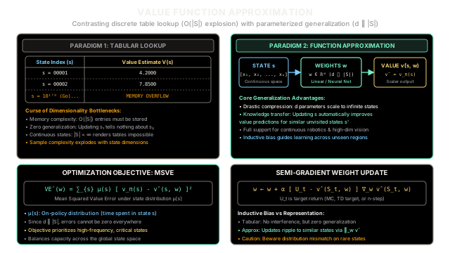
In classical reinforcement learning, foundational algorithms like TD(0), Q-learning, and SARSA represent value functions using tabular lookup tables. In a tabular setting, every discrete state $s$ possesses its own dedicated memory slot $V(s)$ or $Q(s, a)$ . While mathematically transparent and guaranteed to converge without representational bias, tabular methods suffer from two fatal limitations in practical applications:

The Curse of Dimensionality: Tabular memory requirements scale as $\mathcal{O}(|\mathcal{S}|)$ . In simple gridworlds with 20 states, a table is trivial. But in the game of Backgammon ( $10^{20}$ states), Chess ( $10^{47}$ states), or Go ( $10^{170}$ states), storing an explicit table exceeds the number of atoms in the observable universe. In continuous state spaces—such as robotic arm angles, autonomous vehicle LIDAR point clouds, or financial asset prices—the number of possible states is uncountably infinite ( $|\mathcal{S}| = \infty$ ), rendering table allocation fundamentally impossible.
Zero Generalization: Tabular lookup treats every state as an isolated, orthogonal island. If an autonomous car visits state $S_1$ (driving 60.00 mph in the center lane) and learns that this state has high value, an exact tabular agent learns absolutely nothing about state $S_2$ (driving 60.01 mph in the center lane). Because $S_2$ is a different memory key, its table entry remains completely uninitialized. An agent would have to experience every possible micro-variation of the physical universe before making an informed decision.

Value function approximation solves this fundamental bottleneck. Instead of memorizing values in an exhaustive lookup table, the agent approximates the true value function $v_\pi(s)$ or $q_\pi(s, a)$ using a parameterized functional form governed by a compact weight vector $\mathbf{w} \in \mathbb{R}^d$ , where the number of parameters $d$ is exponentially smaller than the number of states ( $d \ll |\mathcal{S}|$ ):

$\hat{v}(s, \mathbf{w}) \approx v_\pi(s)$

By tying the values of all states to a shared parameter vector $\mathbf{w}$ , updating the weights following a transition at state $s$ automatically adjusts the predicted values of similar, unvisited states. Value function approximation transforms reinforcement learning from a problem of rote memorization into a problem of inductive generalization.

Think of It Like This

Predicting House Prices Across a Metropolitan Area

Imagine you are hired as a real estate appraiser to estimate property values across a metropolitan area of two million residences:

The Tabular Approach (Exhaustive Property Spreadsheet): You build an enormous spreadsheet containing two million distinct rows—one for every single street address in the city. When a house at 742 Evergreen Terrace sells for $450,000, you write $450,000 into row 742. However, if a buyer asks you to appraise 744 Evergreen Terrace (the identical house next door that has not sold in fifty years), your tabular spreadsheet outputs zero. You refuse to provide an estimate because you have never personally observed a transaction at that exact street address.
The Function Approximation Approach (Hedonic Pricing Model): Instead of memorizing addresses, you identify key structural features: square footage ( $x_1$ ), number of bedrooms ( $x_2$ ), and school district rating ( $x_3$ ). You fit a parameterized valuation formula: $\text{Price} \approx w_1 \cdot \text{sqft} + w_2 \cdot \text{bedrooms} + w_3 \cdot \text{school\_rating}$ When 742 Evergreen Terrace sells for $450,000, you adjust your parameter weights $\mathbf{w} = [w_1, w_2, w_3]^T$ . That single update instantly updates your price estimates for 744 Evergreen Terrace, the houses across the street, and similar homes across the entire county—even homes that were built yesterday and have never appeared in historical sales records.

Where the analogy breaks down: Real estate regression models are typically trained offline on static historical datasets with independent and identically distributed (i.i.d.) observations. In reinforcement learning, the function approximator updates online while the agent actively navigates the world. As the policy improves, the distribution of visited states shifts dynamically, creating non-stationary target distributions and temporal bootstrapping dependencies.

How It Actually Works

Parameterized Representation and Inductive Generalization

Value function approximation formalizes value estimation as a supervised-like regression problem, but adapts it to the online, non-stationary realities of reinforcement learning.

1. The Parameterized Value Function

Let $s \in \mathcal{S}$ denote a state, and let $\mathbf{w} \in \mathbb{R}^d$ denote a finite parameter vector where $d \ll |\mathcal{S}|$ . The approximate value is denoted:

$\hat{v}(s, \mathbf{w}) \approx v_\pi(s)$

The approximator can be:

Linear Function Approximation: $\hat{v}(s, \mathbf{w}) \doteq \mathbf{w}^T \mathbf{x}(s) = \sum_{i=1}^d w_i x_i(s)$ , where $\mathbf{x}(s) \in \mathbb{R}^d$ is a feature vector extracted from state $s$ (e.g., via tile coding, polynomial bases, or radial basis functions).
Non-Linear Function Approximation: Multi-layer neural networks (e.g., Deep Q-Networks), where $\mathbf{w}$ represents all connection weights and biases across convolutional and dense layers.

2. The Optimization Objective: Mean Squared Value Error

Because the number of parameters $d$ is far smaller than the number of states ( $d \ll |\mathcal{S}|$ ), it is mathematically impossible for $\hat{v}(s, \mathbf{w})$ to equal the true value $v_\pi(s)$ for every state simultaneously. Improving the approximation at one state inevitably alters the approximation at other states.

We must therefore specify a trade-off criterion. The canonical objective in reinforcement learning is the Mean Squared Value Error, denoted $\overline{\text{VE}}(\mathbf{w})$ :

$\overline{\text{VE}}(\mathbf{w}) \doteq \sum_{s \in \mathcal{S}} \mu(s) \left[ v_\pi(s) - \hat{v}(s, \mathbf{w}) \right]^2$

where:

$\mu(s) \ge 0$ is the on-policy state distribution, satisfying $\sum_{s} \mu(s) = 1$ .
$\mu(s)$ represents the fraction of time steps the agent spends in state $s$ under policy $\pi$ in continuing tasks, or normalized discounted visitation frequency in episodic tasks.

The state weighting $\mu(s)$ is vital: it dictates that the function approximator should prioritize representational accuracy on states that the agent visits frequently, while tolerating larger errors on states that the agent rarely or never encounters.

3. Semi-Gradient Stochastic Updates

In stochastic gradient descent (SGD), the weight vector updates in the direction of steepest descent of the squared error for an observed state $S_t$ :

$\mathbf{w}_{t+1} = \mathbf{w}_t - \frac{1}{2} \alpha \nabla_{\mathbf{w}} \left[ v_\pi(S_t) - \hat{v}(S_t, \mathbf{w}_t) \right]^2 = \mathbf{w}_t + \alpha \left[ v_\pi(S_t) - \hat{v}(S_t, \mathbf{w}_t) \right] \nabla_{\mathbf{w}} \hat{v}(S_t, \mathbf{w}_t)$

where $\alpha > 0$ is the step size.

In reinforcement learning, the true target value $v_\pi(S_t)$ is unknown. We substitute an empirical target $U_t$ :

In Monte Carlo, $U_t \doteq G_t$ (the unbiased full return). Because $G_t$ does not depend on $\mathbf{w}$ , this is a true gradient method.
In TD(0), $U_t \doteq R_{t+1} + \gamma \hat{v}(S_{t+1}, \mathbf{w}_t)$ (the one-step bootstrapped target). Because the target itself depends on the current weight vector $\mathbf{w}_t$ , the gradient of the target with respect to $\mathbf{w}$ is ignored. This is termed a semi-gradient method:

$\mathbf{w}_{t+1} = \mathbf{w}_t + \alpha \left[ R_{t+1} + \gamma \hat{v}(S_{t+1}, \mathbf{w}_t) - \hat{v}(S_t, \mathbf{w}_t) \right] \nabla_{\mathbf{w}} \hat{v}(S_t, \mathbf{w}_t)$

4. Tabular Lookup vs. Function Approximation Trade-Offs

Property	Tabular Lookup	Value Function Approximation
Memory Footprint	$\mathcal{O}(\\|\mathcal{S}\\|)$ — explodes with state dimensions	$\mathcal{O}(d)$ where $d \ll \\|\mathcal{S}\\|$ — compact parameter vector
Continuous States	Impossible without arbitrary hard discretization	Fully native via continuous feature vectors
Generalization	Zero (updates to $s$ never affect $s'$ )	High (updates ripple to similar states via feature overlap)
Representational Bias	Zero (can represent any arbitrary mapping)	Introduces inductive bias defined by approximator family
Convergence Guarantees	Exact convergence to $v_\pi$ under standard conditions	Converges to bounded subspace near projection of $v_\pi$

Worked numerical example

To observe generalization directly, let us compare a tabular update against a 2-feature linear parameter update on a single experience transition.

Setup

Suppose an agent operates in a continuous state space where states are represented by two features:

State $S_A$ : $\mathbf{x}(S_A) = [1.0, 0.5]^T$
State $S_B$ (a similar, unvisited state): $\mathbf{x}(S_B) = [1.0, 0.6]^T$

Suppose initial values are zero everywhere:

Tabular: $V(S_A) = 0.0, V(S_B) = 0.0$
Linear Approximator: $\hat{v}(s, \mathbf{w}) = \mathbf{w}^T \mathbf{x}(s) = w_1 x_1 + w_2 x_2$ with $\mathbf{w} = [0.0, 0.0]^T$

The agent visits state $S_A$ and observes an empirical target return $U = 10.0$ .

1. The Tabular Update (Learning Rate $\alpha = 0.5$ )

The tabular update rule updates only the memory bucket corresponding to $S_A$ :

$V(S_A) \leftarrow V(S_A) + \alpha \left[ U - V(S_A) \right] = 0.0 + 0.5 \times (10.0 - 0.0) = 5.0000$

Now inspect the value of the unvisited state $S_B$ : $V(S_B) = 0.0000$

Tabular Result: $S_B$ remains completely uninitialized. Despite being nearly identical to $S_A$ , it receives zero knowledge transfer.

2. The Linear Function Approximation Update (Step Size $\alpha = 0.4$ )

The initial prediction at $S_A$ is: $\hat{v}(S_A, \mathbf{w}) = 0.0 \times 1.0 + 0.0 \times 0.5 = 0.0000$

The prediction error is: $\delta = U - \hat{v}(S_A, \mathbf{w}) = 10.0 - 0.0 = 10.0000$

The gradient with respect to $\mathbf{w}$ is simply the feature vector: $\nabla_{\mathbf{w}} \hat{v}(S_A, \mathbf{w}) = \mathbf{x}(S_A) = \begin{bmatrix} 1.0 \\ 0.5 \end{bmatrix}$

We apply the stochastic gradient update: $\mathbf{w} \leftarrow \mathbf{w} + \alpha \delta \nabla_{\mathbf{w}} \hat{v}(S_A, \mathbf{w}) = \begin{bmatrix} 0.0 \\ 0.0 \end{bmatrix} + 0.4 \times 10.0 \times \begin{bmatrix} 1.0 \\ 0.5 \end{bmatrix} = \begin{bmatrix} 0.0 \\ 0.0 \end{bmatrix} + 4.0 \times \begin{bmatrix} 1.0 \\ 0.5 \end{bmatrix} = \begin{bmatrix} 4.0 \\ 2.0 \end{bmatrix}$

Now evaluate both states under the updated weight vector $\mathbf{w} = [4.0, 2.0]^T$ :

At visited state $S_A$ : $\hat{v}(S_A, \mathbf{w}) = (4.0 \times 1.0) + (2.0 \times 0.5) = 4.0 + 1.0 = 5.0000$
At unvisited state $S_B$ : $\hat{v}(S_B, \mathbf{w}) = (4.0 \times 1.0) + (2.0 \times 0.6) = 4.0 + 1.2 = 5.2000$

Function Approximation Result: Even though the agent has never encountered $S_B$ , its estimated value updated immediately from $0.0000$ to $5.2000$ . The shared parameter vector generalized the experience smoothly across continuous feature space.

Code

The following self-contained Python script demonstrates the fundamental failure of tabular memory on continuous state spaces compared to the smooth generalization achieved by a linear value function approximator:

1import math2from typing import Dict, List, Tuple3
4
5class TabularValueFunction:6    """Exact table lookup value function representation."""7
8    def __init__(self) -> None:9        self.table: Dict[Tuple[float, ...], float] = {}10
11    def get(self, state: Tuple[float, ...]) -> float:12        """Retrieve value for an exact state tuple, returning 0.0 if unvisited."""13        return self.table.get(state, 0.0)14
15    def update(self, state: Tuple[float, ...], target: float, alpha: float) -> float:16        """Update tabular entry toward target."""17        current = self.get(state)18        error = target - current19        self.table[state] = current + alpha * error20        return error21
22
23class LinearValueApproximator:24    """Linear value function approximator: v_hat(s, w) = w^T x(s)."""25
26    def __init__(self, num_features: int) -> None:27        self.weights: List[float] = [0.0] * num_features28
29    def predict(self, features: List[float]) -> float:30        """Compute inner product between weights and feature vector."""31        return sum(w * x for w, x in zip(self.weights, features))32
33    def update(self, features: List[float], target: float, alpha: float) -> float:34        """Semi-gradient SGD update: w <- w + alpha * (target - v_hat) * grad."""35        prediction = self.predict(features)36        error = target - prediction37        # For linear models, grad_w v_hat(s, w) = features38        for i in range(len(self.weights)):39            self.weights[i] += alpha * error * features[i]40        return error41
42
43def run_vfa_demonstration() -> None:44    # Part 1: Worked Numerical Comparison (State A vs State B)45    state_a = (1.0, 0.5)46    state_b = (1.0, 0.6)47    target_val = 10.048
49    tabular = TabularValueFunction()50    tabular.update(state_a, target_val, alpha=0.5)51    v_tab_a = tabular.get(state_a)52    v_tab_b = tabular.get(state_b)53
54    linear = LinearValueApproximator(num_features=2)55    linear.update(list(state_a), target_val, alpha=0.4)56    v_lin_a = linear.predict(list(state_a))57    v_lin_b = linear.predict(list(state_b))58
59    print("--- Single-Step Generalization Comparison ---")60    print(f"Tabular V(S_A visited):   {v_tab_a:.4f}")61    print(f"Tabular V(S_B unvisited): {v_tab_b:.4f} (Zero generalization!)")62    print(f"Linear w parameters:      [{linear.weights[0]:.4f}, {linear.weights[1]:.4f}]")63    print(f"Linear V(S_A visited):    {v_lin_a:.4f}")64    print(f"Linear V(S_B unvisited):  {v_lin_b:.4f} (Generalizes from shared weights!)")65
66    assert abs(v_tab_a - 5.0) < 1e-567    assert abs(v_tab_b - 0.0) < 1e-568    assert abs(v_lin_a - 5.0) < 1e-569    assert abs(v_lin_b - 5.2) < 1e-570
71    # Part 2: Continuous State Space Generalization Experiment72    # True underlying value function: v*(s) = 2.0 * s + 1.0 on continuous s in [0, 10]73    def true_value(s: float) -> float:74        return 2.0 * s + 1.075
76    training_states = [1.0, 3.0, 5.0, 8.0]77    unvisited_test_states = [2.0, 4.0, 6.5, 9.0]78
79    # Train tabular model on visited states80    tab_model = TabularValueFunction()81    for s in training_states:82        tab_model.update((s,), true_value(s), alpha=1.0)83
84    # Train linear model on visited states (features: [bias=1.0, state=s])85    lin_model = LinearValueApproximator(num_features=2)86    for _ in range(200):87        for s in training_states:88            lin_model.update([1.0, s], true_value(s), alpha=0.02)89
90    # Evaluate Root Mean Squared Error (RMSE) on unvisited test states91    tab_test_errors = [92        abs(tab_model.get((s,)) - true_value(s)) for s in unvisited_test_states93    ]94    rmse_tabular = math.sqrt(sum(e**2 for e in tab_test_errors) / len(unvisited_test_states))95
96    lin_test_errors = [97        abs(lin_model.predict([1.0, s]) - true_value(s)) for s in unvisited_test_states98    ]99    rmse_linear = math.sqrt(sum(e**2 for e in lin_test_errors) / len(unvisited_test_states))100
101    print("\n--- Continuous State Space Generalization Test ---")102    print(f"Tabular RMSE on unvisited states: {rmse_tabular:.4f}")103    print(f"Linear RMSE on unvisited states:  {rmse_linear:.4f}")104
105    # Tabular completely fails on unseen continuous points; linear generalizes with near-zero error106    assert rmse_tabular > 10.0107    assert rmse_linear < 0.05108
109
110if __name__ == "__main__":111    run_vfa_demonstration()112
113# -> Expected output:114# -> --- Single-Step Generalization Comparison ---115# -> Tabular V(S_A visited):   5.0000116# -> Tabular V(S_B unvisited): 0.0000 (Zero generalization!)117# -> Linear w parameters:      [4.0000, 2.0000]118# -> Linear V(S_A visited):    5.0000119# -> Linear V(S_B unvisited):  5.2000 (Generalizes from shared weights!)120# -> 121# -> --- Continuous State Space Generalization Test ---122# -> Tabular RMSE on unvisited states: 12.8744123# -> Linear RMSE on unvisited states:  0.0022

Watch Out For

The State Distribution Mismatch: Starving Rare but Critical States

Because a function approximator has limited capacity ( $d \ll |\mathcal{S}|$ ), it cannot fit all states with equal fidelity. By definition, optimizing the Mean Squared Value Error objective $\overline{\text{VE}}(\mathbf{w}) = \sum_s \mu(s) [v_\pi(s) - \hat{v}(s, \mathbf{w})]^2$ allocates representational precision strictly in proportion to state visitation frequency $\mu(s)$ .

The Symptom: If the behavioral distribution $\mu(s)$ is heavily skewed toward safe, routine states (such as cruising straight on a highway), the function approximator aggressively minimizes loss on those high-frequency states. In doing so, it happily sacrifices accuracy on rare, low-frequency states—such as emergency skid recovery, rare cliff edges, or black swan financial crashes. When the agent inevitably encounters one of these rare states, its value predictions are wildly erroneous, triggering catastrophic failure modes despite low global training loss.

The Fix:

Prioritized Replay Buffers: In deep reinforcement learning, sample transitions proportional to TD error magnitude rather than uniform historical frequency, ensuring rare high-surprise states receive frequent gradient updates.
Importance Sampling Adjustments: When learning off-policy, reweight gradient steps by the Radon-Nikodym derivative $\frac{\pi(a \mid s)}{b(a \mid s)}$ to prevent behavioral data distributions from corrupting the target policy's objective.
Localized Feature Architectures: In linear methods, use local basis representations like tile coding or radial basis functions (RBFs) so that updates to frequent states do not overwrite or interfere with weights assigned to distant regions of the state space.

The Quick Version

Overcoming Tabular Limits: Value function approximation replaces discrete $\mathcal{O}(|\mathcal{S}|)$ lookup tables with a parameterized function $\hat{v}(s, \mathbf{w})$ where $d \ll |\mathcal{S}|$ , enabling RL to scale to infinite continuous state spaces.
Inductive Generalization: Updating a shared weight vector $\mathbf{w}$ using experience from state $s$ automatically refines value estimates for similar, unvisited states across the state space.
Weighted Trade-Off Objective: Because $d$ parameters cannot fit all states perfectly, the Mean Squared Value Error objective weights errors by the on-policy visitation distribution $\mu(s)$ to prioritize high-frequency states.
Semi-Gradient Learning: When updating value weights with bootstrapped targets (like TD(0)), the algorithm ignores the target's dependency on $\mathbf{w}$ , forming a semi-gradient update that converges near the projection of $v_\pi$ .