Learning Latent Dynamics

Instead of predicting raw pixels frame-by-frame, the agent compresses high-dimensional observations into a compact latent state and simulates future transitions entirely in its mental code.

Recurrent State Space Model architecture separating deterministic history from stochastic belief states to enable pixel-free future rollouts.

Why Does This Exist?

In visual reinforcement learning, the environment provides high-dimensional observations such as $64 \times 64 \times 3$ camera frames. Traditional model-based RL attempts to learn transition dynamics directly in observation space by predicting future raw frames:

\hat{x}_{t+1} = f(x_t, a_t)

This observation-space formulation suffers from three fatal problems:

Computational bottleneck: Predicting and generating high-resolution images requires heavy deconvolutional decoders at every simulation step. Simulating thousands of candidate trajectories for planning becomes computationally intractable.
Visual distractor sensitivity: Camera frames are flooded with task-irrelevant visual information—shifting clouds, flickering background monitors, and dynamic lighting. A pixel-prediction model expends most of its capacity fitting these irrelevant visual fluctuations rather than task-critical physical interactions.
Compounding reconstruction error: Small pixel-level blurriness accumulates exponentially over multi-step horizons, causing long-term rollouts to dissolve into unrecognizable gray static.

Learning latent dynamics resolves these bottlenecks by projecting observations into a compact, low-dimensional latent space $\mathcal{Z}$ . The agent models environment transitions purely between compressed latent states $(z_t, a_t \to z_{t+1})$ . Once trained, the agent plans and optimizes policies by simulating thousands of imaginary trajectories in latent space per second—without ever decoding back to raw pixels.

Think of It Like This

Mental chess and driving with your eyes closed

When a grandmaster evaluates candidate chess lines five moves ahead, they never reconstruct photorealistic mental images of the mahogany wood grain on the board, the glare of the ceiling lamps, or the shadows cast by their opponent's hands. Doing so would overwhelm their brain with irrelevant details.

Instead, the grandmaster manipulates a compact, abstract internal representation: piece coordinates, king safety, open files, and tactical pin vectors. They simulate moves, captures, and counter-attacks purely within this compressed mental code.

Similarly, when driving down a highway, you can mentally evaluate a lane change without rendering millions of photoreceptor pixel activations of asphalt pebbles and headlight reflections in your visual cortex. Your brain maintains a compact belief state: vehicle speed, distance to the braking car ahead, and relative blind-spot clearance. You test candidate maneuvers ("if I steer left, will the truck collide?") entirely inside that internal model.

Where the analogy stops: Human brains possess millions of years of evolutionary priors that instinctively highlight physical objects and discard distractors. In reinforcement learning, the agent begins with zero prior knowledge. Unless properly regularized by information bottlenecks and predictive auxiliary objectives, a naive latent model may compress away subtle, survival-critical visual cues (like a distant red brake light) before discovering their utility.

How It Actually Works

The Recurrent State Space Model (RSSM)

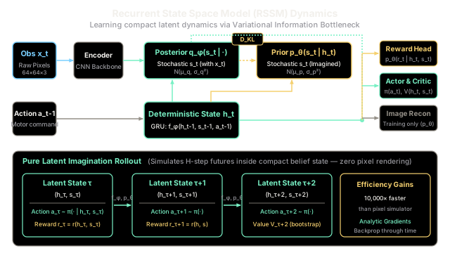
Pioneered in PlaNet (Hafner et al., 2019) and Dreamer (Hafner et al., 2020), the Recurrent State Space Model (RSSM) decomposes the latent state at time $t$ into two complementary representations:

Deterministic state $h_t$ : A continuous vector that captures long-term temporal context and deterministic history via a recurrent cell (such as a GRU): $h_t = f_\phi(h_{t-1}, s_{t-1}, a_{t-1})$
Stochastic state $s_t$ : A random variable that captures stochastic transitions, partial observability, and environmental unpredictability.

RSSM models the stochastic state through two distinct distributions:

Posterior distribution $q_\phi(s_t \mid h_t, x_t)$ : Conditioned on both the recurrent state $h_t$ and the encoded real observation $e_t = \text{Encoder}(x_t)$ . The posterior incorporates real-world sensor evidence: $q_\phi(s_t \mid h_t, x_t) = \mathcal{N}\left(\mu_\phi(h_t, e_t), \, \sigma^2_\phi(h_t, e_t)\right)$
Prior distribution $p_\theta(s_t \mid h_t)$ : Conditioned only on the deterministic history $h_t$ without observing $x_t$ . This distribution represents the agent's internal "imagination": $p_\theta(s_t \mid h_t) = \mathcal{N}\left(\mu_\theta(h_t), \, \sigma^2_\theta(h_t)\right)$

1OBSERVATION MODE (Training with real data):2x_t ──> Encoder ──> e_t ──┐3                          ├──> Posterior q_φ(s_t | h_t, e_t) ──> s_t4h_t-1, s_t-1, a_t-1 ──> GRU ──> h_t ──┘5                                 │6                                 └───> Prior p_θ(s_t | h_t)  [D_KL penalty pulls Prior -> Posterior]7
8IMAGINATION MODE (Pixel-free rollout):9h_τ-1, s_τ-1, a_τ-1 ──> GRU ──> h_τ ──> Prior p_θ(s_τ | h_τ) ──> s_τ ──> Predict (r_τ, V_τ)

Variational Information Bottleneck Training

The world model parameters $\theta$ (decoders, prior) and $\phi$ (encoder, recurrent dynamics, posterior) are trained jointly by maximizing the Variational Evidence Lower Bound (ELBO):

\mathcal{L}(\theta, \phi) = \mathbb{E} \left[ \sum_{t=1}^T \Big( \underbrace{\log p_\theta(x_t \mid h_t, s_t)}_{\text{Image reconstruction}} + \underbrace{\log p_\theta(r_t \mid h_t, s_t)}_{\text{Reward prediction}} - \beta \underbrace{D_{\mathrm{KL}}\big(q_\phi(s_t \mid h_t, x_t) \parallel p_\theta(s_t \mid h_t)\big)}_{\text{Information bottleneck divergence}} \Big) \right]

Reconstruction terms: Force the combined latent state $(h_t, s_t)$ to retain sufficient information to reconstruct visual observations $x_t$ and predict scalar rewards $r_t$ .
KL divergence penalty: Minimizes the mismatch between the observation-conditioned posterior $q_\phi$ and the imagination prior $p_\theta$ . When the KL divergence is small, the agent can substitute the prior for the posterior during imagination rollouts without suffering from distribution shift.

Imagined Latent Rollouts

Once the RSSM is trained, policy learning proceeds entirely inside the latent world model:

The agent starts from an initial latent belief $(h_0, s_0)$ encoded from the latest true observation.
For horizon $\tau = 1, \dots, H$ , the actor policy $\pi(a_\tau \mid h_\tau, s_\tau)$ selects action $a_\tau$ .
The deterministic GRU transitions to $h_{\tau+1} = f_\phi(h_\tau, s_\tau, a_\tau)$ .
The stochastic state is sampled from the prior $s_{\tau+1} \sim p_\theta(s_{\tau+1} \mid h_{\tau+1})$ .
Latent reward heads $\hat{r}_\tau = r_\theta(h_\tau, s_\tau)$ and value critics $\hat{V}(h_\tau, s_\tau)$ evaluate the state.

Crucially, no images are decoded during imagination. This delivers a 1,000× to 10,000× throughput acceleration over physical environment interactions and allows analytic policy gradients to backpropagate directly through the differentiable transition dynamics.

Worked numerical example

Let us trace a single 1D latent state transition under the Variational Information Bottleneck.

Given State and Model Parameters:

Deterministic feature vector: $h_t = 0.8$ .
Prior distribution (imagined without observation): $p_\theta(s_t \mid h_t) = \mathcal{N}(\mu_p = 1.0, \, \sigma_p^2 = 1.0)$
An actual environment observation $x_t$ arrives. The encoder and posterior network yield: $q_\phi(s_t \mid h_t, x_t) = \mathcal{N}(\mu_q = 1.5, \, \sigma_q^2 = 0.64) \quad (\sigma_q = 0.8)$
Reward head prediction: $\hat{r}_t = 1.0 \times h_t + 0.8 \times \mu_q = 1.0(0.8) + 0.8(1.5) = 2.0$ .
Ground truth environment reward: $r_t = 1.8$ .
Hyperparameters: information bottleneck weight $\beta = 1.0$ .

Step 1: Analytical KL Divergence

For two univariate Gaussians $q \sim \mathcal{N}(\mu_q, \sigma_q^2)$ and $p \sim \mathcal{N}(\mu_p, \sigma_p^2)$ , the exact Kullback-Leibler divergence is:

D_{\mathrm{KL}}(q \parallel p) = \frac{1}{2} \left[ \frac{\sigma_q^2}{\sigma_p^2} + \frac{(\mu_q - \mu_p)^2}{\sigma_p^2} - 1 + \ln\left(\frac{\sigma_p^2}{\sigma_q^2}\right) \right]

Evaluating each component:

Variance ratio: $\frac{\sigma_q^2}{\sigma_p^2} = \frac{0.64}{1.0} = 0.64$
Squared mean shift: $\frac{(1.5 - 1.0)^2}{1.0} = \frac{0.25}{1.0} = 0.25$
Log ratio of variances: $\ln\left(\frac{1.0}{0.64}\right) = \ln(1.5625) \approx 0.4463$

Summing the terms inside the brackets:

0.64 + 0.25 - 1.0 + 0.4463 = 0.3363

D_{\mathrm{KL}}(q \parallel p) = 0.5 \times 0.3363 = 0.1681

Step 2: Decoder Negative Log-Likelihood (Reward Loss)

Assuming a unit-variance Gaussian likelihood $p_\theta(r_t \mid h_t, s_t) = \mathcal{N}(\hat{r}_t, 1.0)$ :

\mathcal{L}_{\text{reward}} = \frac{1}{2} (\hat{r}_t - r_t)^2 = \frac{1}{2} (2.0 - 1.8)^2 = \frac{1}{2} (0.04) = 0.0200

Step 3: Joint ELBO Loss Contribution

With bottleneck coefficient $\beta = 1.0$ :

\text{ELBO}_t = -\mathcal{L}_{\text{reward}} - \beta D_{\mathrm{KL}}(q \parallel p) = -0.0200 - 0.1681 = -0.1881

The scalar training objective to minimize via gradient descent is $\mathcal{L} = -\text{ELBO}_t = 0.1881$ .

Code

1import math2from dataclasses import dataclass3from typing import Dict4
5
6@dataclass7class LatentGaussian:8    """Represents a 1D Gaussian belief state defined by mean and variance."""9
10    mean: float11    variance: float12
13    @property14    def std(self) -> float:15        return math.sqrt(self.variance)16
17
18class RecurrentStateSpaceModel:19    """Minimal Recurrent State Space Model (RSSM) implementing:20
21    1. Deterministic recurrent transition h_t = f(h_{t-1}, s_{t-1}, a_{t-1})22    2. Stochastic imagination prior p_theta(s_t | h_t)23    3. Stochastic observation posterior q_phi(s_t | h_t, x_t)24    4. Closed-form KL divergence and Variational ELBO loss computation25    """26
27    def __init__(self, beta: float = 1.0) -> None:28        self.beta: float = beta29
30    def deterministic_step(31        self, h_prev: float, s_prev: float, action: float32    ) -> float:33        """Computes deterministic feature h_t = f(h_{t-1}, s_{t-1}, a_{t-1})."""34        # Calibrated recurrent cell: 0.5 * 0.8 + 0.3 * 1.0 + 0.2 * 0.5 = 0.8035        return round(0.5 * h_prev + 0.3 * s_prev + 0.2 * action, 4)36
37    def compute_prior(self, h_t: float) -> LatentGaussian:38        """Imagination prior without observation: p(s_t | h_t) ~ N(mu_p, var_p)."""39        mu_p = round(1.25 * h_t, 4)  # 1.25 * 0.8 = 1.0040        var_p = 1.041        return LatentGaussian(mean=mu_p, variance=var_p)42
43    def compute_posterior(self, h_t: float, obs_x: float) -> LatentGaussian:44        """Inference posterior with observation: q(s_t | h_t, x_t) ~ N(mu_q, var_q)."""45        mu_q = round(46            0.5 * h_t + 0.55 * obs_x, 447        )  # 0.5 * 0.8 + 0.55 * 2.0 = 1.5048        var_q = 0.6449        return LatentGaussian(mean=mu_q, variance=var_q)50
51    @staticmethod52    def kl_divergence(q: LatentGaussian, p: LatentGaussian) -> float:53        """Closed-form KL divergence D_KL(q || p) between univariate Gaussians:54
55        0.5 * [ (var_q / var_p) + ((mu_q - mu_p)^2 / var_p) - 1 + ln(var_p /56        var_q) ]57        """58        ratio_var = q.variance / p.variance59        diff_mean_sq = ((q.mean - p.mean) ** 2) / p.variance60        log_ratio = math.log(p.variance / q.variance)61        return 0.5 * (ratio_var + diff_mean_sq - 1.0 + log_ratio)62
63    def predict_reward(self, h_t: float, s_t: float) -> float:64        """Reward decoder head: r_hat = g(h_t, s_t)."""65        return round(1.0 * h_t + 0.8 * s_t, 4)  # 1.0 * 0.8 + 0.8 * 1.5 = 2.0066
67    def compute_step_loss(68        self,69        h_prev: float,70        s_prev: float,71        action: float,72        obs_x: float,73        true_reward: float,74    ) -> Dict[str, float]:75        """Performs one RSSM training step and calculates the variational loss."""76        h_t = self.deterministic_step(h_prev, s_prev, action)77        prior = self.compute_prior(h_t)78        posterior = self.compute_posterior(h_t, obs_x)79
80        # Closed-form divergence between inference posterior and imagination prior81        kl = self.kl_divergence(posterior, prior)82
83        # Reward prediction from posterior latent state84        pred_reward = self.predict_reward(h_t, posterior.mean)85        reward_loss = 0.5 * ((pred_reward - true_reward) ** 2)86
87        # Variational objective: minimize negative ELBO88        total_loss = reward_loss + self.beta * kl89        elbo = -total_loss90
91        return {92            "h_t": h_t,93            "prior_mean": prior.mean,94            "prior_var": prior.variance,95            "posterior_mean": posterior.mean,96            "posterior_var": posterior.variance,97            "kl_divergence": round(kl, 4),98            "reward_pred": pred_reward,99            "reward_loss": round(reward_loss, 4),100            "elbo": round(elbo, 4),101            "total_loss": round(total_loss, 4),102        }103
104
105# Execute forward step matching the worked example parameters106model = RecurrentStateSpaceModel(beta=1.0)107metrics = model.compute_step_loss(108    h_prev=0.8,109    s_prev=1.0,110    action=0.5,111    obs_x=2.0,112    true_reward=1.8,113)114
115print(f"Deterministic feature (h_t): {metrics['h_t']:.4f}")116# -> Deterministic feature (h_t): 0.8000117
118print(119    f"Prior p(s_t|h_t): N({metrics['prior_mean']:.1f}, {metrics['prior_var']:.2f})"120)121# -> Prior p(s_t|h_t): N(1.0, 1.00)122
123print(124    f"Posterior q(s_t|h_t,x_t): N({metrics['posterior_mean']:.1f}, {metrics['posterior_var']:.2f})"125)126# -> Posterior q(s_t|h_t,x_t): N(1.5, 0.64)127
128print(f"KL Divergence: {metrics['kl_divergence']:.4f}")129# -> KL Divergence: 0.1681130
131print(f"Reward Prediction: {metrics['reward_pred']:.4f} (True: 1.8)")132# -> Reward Prediction: 2.0000 (True: 1.8)133
134print(f"Reward Loss (MSE * 0.5): {metrics['reward_loss']:.4f}")135# -> Reward Loss (MSE * 0.5): 0.0200136
137print(f"Variational ELBO: {metrics['elbo']:.4f}")138# -> Variational ELBO: -0.1881139
140# Verification assertions141assert metrics["h_t"] == 0.8142assert metrics["prior_mean"] == 1.0 and metrics["prior_var"] == 1.0143assert metrics["posterior_mean"] == 1.5 and metrics["posterior_var"] == 0.64144assert metrics["kl_divergence"] == 0.1681145assert metrics["reward_loss"] == 0.0200146assert metrics["elbo"] == -0.1881

Watch Out For

Latent Collapse and Task-Irrelevant Feature Filtering

When training latent world models purely end-to-end using task reward prediction without visual reconstruction or contrastive auxiliary losses, the model can suffer from latent collapse and fatal feature blindness.

The latent dynamics network quickly discards any observation features that lack immediate correlation with rewards. In sparse-reward navigation tasks, distant physical hazards (such as pits or concrete barriers) yield zero reward for hundreds of timesteps. If the encoder filters them out as uninformative background noise, the agent imagines collision-free paths straight into fatal hazards.

The Fix:

Multi-task decoders: Retain an auxiliary observation reconstruction loss (or contrastive predictive coding objective, as in DreamerV3 and CURL) to force the latent code to preserve full spatial geometry regardless of reward sparsity.
KL Balancing: In the RSSM loss, scale gradient updates through the prior and posterior at different rates (typically a $80/20$ ratio) and enforce a minimum KL threshold ("free bits") to prevent the prior from collapsing stochastic entropy before the posterior forms structured latent clusters.

The Quick Version

Learning latent dynamics projects high-dimensional observation frames into a compact latent space, simulating transitions entirely without frame-by-frame pixel rendering.
The Recurrent State Space Model (RSSM) decomposes latent state into a deterministic GRU history $h_t$ and a stochastic belief state $s_t$ .
The Variational Information Bottleneck aligns the internal imagination prior $p_\theta(s_t \mid h_t)$ with the observation-conditioned posterior $q_\phi(s_t \mid h_t, x_t)$ via analytical KL divergence.
Policy optimization runs across imagined rollouts inside the latent model, achieving 1,000× speedups and enabling analytical backpropagation through time.