Planning with Learned Models

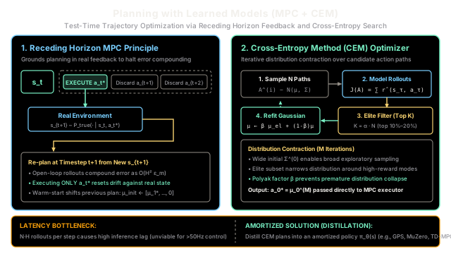
Planning with learned models optimizes action sequences at test time by simulating trajectories through an internal world model. By executing only the first action of an optimized plan and immediately re-planning, Model Predictive Control prevents simulation drift from compounding into real-world failure.

Model Predictive Control and Cross-Entropy Method trajectory optimization rolling out candidates through learned dynamics with receding horizon replanning.

Why Does This Exist?

In classical model-free reinforcement learning, an agent memorizes decisions through a parameterized policy network $\pi_\theta(a \mid s)$ . Training this network requires millions of trials, and the resulting weights are rigidly coupled to the exact reward function and dynamics encountered during training. If the target goal shifts at test time, or if an obstacle suddenly blocks a corridor, a model-free actor is blind to the change until thousands of new gradient steps update its weights.

Planning with learned models decouples decision-making from fixed policy parameters. Instead of memorizing which action to take in advance, the agent learns a transition dynamics model $\hat{p}_\theta(s_{t+1} \mid s_t, a_t)$ and reward function $\hat{r}(s_t, a_t)$ . At test time, the agent actively searches for high-return action trajectories inside this internal simulation.

However, naive open-loop trajectory optimization suffers from a fatal pathology: compounding model error. If an agent generates an optimal 30-step action plan using its learned model and executes all 30 steps open-loop, single-step approximation errors $\epsilon_m$ compound quadratically or exponentially over the horizon $\mathcal{O}(H^2 \epsilon_m)$ . By step 10, the physical environment has drifted drastically from the imagined state, and the remaining actions produce catastrophic failures.

Model Predictive Control (MPC) and shooting algorithms like the Cross-Entropy Method (CEM) resolve this vulnerability through the Receding Horizon Principle:

At state $s_t$ , optimize action trajectories across a prospective horizon $H$ .
Execute only the very first action $a_t^*$ .
Discard the remainder of the plan.
Observe the true next environmental state $s_{t+1}$ and re-plan from scratch.

By continuously grounding the optimization in true physical feedback at every single timestep, receding-horizon planning eliminates open-loop drift and provides robust, zero-shot adaptation to arbitrary test-time objectives.

Think of It Like This

Navigating a sailboat through shifting wind gusts

Imagine piloting a high-performance sailboat across an unpredictable channel with choppy waves and shifting wind gusts.

A model-free policy approach is like memorizing a rigid rudder and sail timetable three months before the voyage: "At minute 14, turn rudder 12 degrees starboard; at minute 15, ease the mainsail 4 inches." The instant an unexpected wave knocks the hull off course, the pre-memorized timetable drives the boat directly into the reef.

An MPC and Cross-Entropy Method navigator operates with dynamic foresight:

At every single wave crest, you look ahead across the next 10 seconds (the planning horizon $H$ ).
You mentally simulate 100 hypothetical rudder angles and sail positions (sampling candidate action sequences $A^{(i)} \sim \mathcal{N}(\mu, \Sigma)$ through your learned model of boat dynamics).
You identify the top 10% smoothest, fastest courses through the chop (the Cross-Entropy Method elite candidates).
You refine your planned rudder maneuver by averaging these top candidates (refitting the action distribution $\mu_{\text{elite}}$ ).
Crucially, you only execute the first second of that maneuver ( $a_t^*$ ).
When the boat lands on the next wave crest, you do not blindly follow the remaining 9 seconds of the old calculation. You observe your true GPS position, wind direction, and boat tilt, and re-simulate 100 new prospective courses from scratch.

Where the analogy stops: human sailors use qualitative visual heuristics and physical intuition. An algorithmic MPC controller computes explicit numerical forward integrations through neural networks, evaluating thousands of candidate floating-point tensors within strict millisecond control deadlines.

How It Actually Works

Model Predictive Control and the Cross-Entropy Method

Planning with learned models replaces policy networks with online trajectory optimization via shooting methods.

1       ┌────────────────────────────────────────────────────────┐2       │             MPC Receding Horizon Control Loop          │3       └───────────────────────────┬────────────────────────────┘4                                   │5      ┌────────────────────────────▼────────────────────────────┐6      │  Current Environment State s_t                          │7      └────────────────────────────┬────────────────────────────┘8                                   │9      ┌────────────────────────────▼────────────────────────────┐10      │  Trajectory Optimization (CEM):                         │11      │  Sample N action sequences ~ N(μ, Σ)                    │12      │  Roll out in learned model p̂_θ(s'|s,a) for H steps      │13      │  Filter elite top-K candidates & refit distribution     │14      └────────────────────────────┬────────────────────────────┘15                                   │16         ┌─────────────────────────┴─────────────────────────┐17         │ Optimal Action Sequence: [a_t*, a_{t+1}*, ..., a_{t+H-1}*]18         │19         ▼20┌──────────────────┐               ┌─────────────────────────────────┐21│ EXECUTE ONLY a_t*│ ─────────────►│ Discard a_{t+1}* ... a_{t+H-1}* │22└────────┬─────────┘               └─────────────────────────────────┘23         │24         ▼25┌──────────────────────────┐26│ Physical Environment     │27│ s_{t+1} ~ P_true(·|s, a) │28└────────┬─────────────────┘29         │30         └─────────────────────────► Shift horizon & re-plan from s_{t+1}

1. Shooting Methods and the Receding Horizon Principle

In shooting methods, the decision variables are the sequences of prospective actions over a finite planning horizon $H$ :

A = (a_t, a_{t+1}, \dots, a_{t+H-1}) \in \mathbb{R}^{H \times d_a}

Starting from the current physical state $\hat{s}_t = s_t$ , prospective states are predicted forward sequentially using the learned dynamics model $\hat{p}_\theta$ :

\hat{s}_{\tau+1} = \hat{f}_\theta(\hat{s}_\tau, a_\tau), \quad \tau \in \{t, \dots, t+H-1\}

The trajectory optimization objective seeks the action sequence maximizing the cumulative predicted return:

\max_{a_{t:t+H-1}} J(s_t, a_{t:t+H-1}) = \sum_{\tau=t}^{t+H-1} \gamma^{\tau-t} \hat{r}(\hat{s}_\tau, a_\tau) + \gamma^H \hat{V}_\psi(\hat{s}_{t+H})

where $\hat{V}_\psi$ is an optional terminal value function (used in algorithms like TD-MPC) to account for infinite-horizon returns beyond the planning cutoff $H$ .

Under Model Predictive Control (MPC):

The optimization solves for $A^* = (a_t^*, a_{t+1}^*, \dots, a_{t+H-1}^*)$ .
The agent executes only the first action: $a_t = a_t^*$ .
The remaining actions $a_{t+1:t+H-1}^*$ are discarded.
The environment steps to the true next state: $s_{t+1} \sim P_{\text{true}}(\cdot \mid s_t, a_t^*)$ .
The optimization problem is re-solved at timestep $t+1$ starting from the ground-truth state $s_{t+1}$ .

2. The Cross-Entropy Method (CEM) for Trajectory Optimization

Because learned neural dynamics models create complex, non-convex, and potentially discontinuous reward surfaces, standard gradient ascent on action vectors frequently gets trapped in poor local optima or suffers from exploding/vanishing gradients through time.

The Cross-Entropy Method (CEM) is an evolutionary, derivative-free optimization algorithm that iteratively contracts a sampling distribution around high-performing action sequences.

At each planning timestep $t$ , CEM executes $M$ optimization iterations:

Step 1: Initialize Sampling Distribution

The action sequence distribution is modeled as a factorized Gaussian across the planning horizon:

q^{(0)}(A) = \mathcal{N}\left( \boldsymbol{\mu}^{(0)}, \boldsymbol{\Sigma}^{(0)} \right)

where $\boldsymbol{\mu}^{(0)} \in \mathbb{R}^{H \times d_a}$ is initialized to zeros (or warm-started from the shifted solution of the previous timestep), and $\boldsymbol{\Sigma}^{(0)} = \operatorname{diag}(\boldsymbol{\sigma}^{2(0)})$ is set to broad variance (e.g., $\sigma^2 = 1.0$ ).

Step 2: Candidate Sampling

At iteration $m \in \{0, \dots, M-1\}$ , sample $N$ candidate action sequences:

A^{(i)} \sim \mathcal{N}\left( \boldsymbol{\mu}^{(m)}, \boldsymbol{\Sigma}^{(m)} \right), \quad i \in \{1, \dots, N\}

Each candidate $A^{(i)}$ is clipped to valid physical control bounds $[a_{\min}, a_{\max}]$ .

Step 3: Trajectory Evaluation

Each candidate sequence is simulated through the learned dynamics model $\hat{p}_\theta$ starting from current state $s_t$ , computing its predicted return:

J(A^{(i)}) = \sum_{\tau=0}^{H-1} \gamma^\tau \hat{r}(\hat{s}_\tau^{(i)}, a_\tau^{(i)})

Step 4: Elite Selection

Sort the candidates in descending order of predicted return:

J(A^{(\pi_1)}) \ge J(A^{(\pi_2)}) \ge \dots \ge J(A^{(\pi_N)})

Extract the top $K$ candidates (the elite set $\mathcal{E}$ ), where $K = \lfloor \alpha N \rfloor$ (typically $\alpha \in [0.05, 0.20]$ ):

\mathcal{E} = \left\{ A^{(\pi_1)}, A^{(\pi_2)}, \dots, A^{(\pi_K)} \right\}

Step 5: Refit Distribution Parameters

Compute the empirical sample mean and sample variance of the elite set:

\boldsymbol{\mu}_{\text{elite}} = \frac{1}{K} \sum_{k=1}^K A^{(\pi_k)}

\boldsymbol{\Sigma}_{\text{elite}} = \frac{1}{K} \sum_{k=1}^K \left( A^{(\pi_k)} - \boldsymbol{\mu}_{\text{elite}} \right) \odot \left( A^{(\pi_k)} - \boldsymbol{\mu}_{\text{elite}} \right)

Step 6: Polyak Momentum Smoothing

To prevent the sampling distribution from collapsing prematurely into a narrow sub-optimal spike, update parameters using exponential smoothing factor $\beta \in (0, 1]$ :

\boldsymbol{\mu}^{(m+1)} = \beta \boldsymbol{\mu}_{\text{elite}} + (1 - \beta) \boldsymbol{\mu}^{(m)}

\boldsymbol{\Sigma}^{(m+1)} = \beta \boldsymbol{\Sigma}_{\text{elite}} + (1 - \beta) \boldsymbol{\Sigma}^{(m)}

After $M$ iterations, the mean of the converged distribution at the first timestep is returned as the control action:

a_t^* = \boldsymbol{\mu}_0^{(M)}

Worked numerical example

Let us trace a single CEM refinement step by hand on a 1D control problem ( $d_a = 1$ ) over a planning horizon $H = 2$ .

Population size: $N = 4$ candidate action sequences
Elite fraction: top $K = 2$ candidates ( $\alpha = 0.50$ )
Polyak momentum smoothing: $\beta = 0.80$
Initial prior distribution at iteration $m = 0$ : $\boldsymbol{\mu}^{(0)} = \begin{bmatrix} 0.0 \\ 0.0 \end{bmatrix}, \quad \boldsymbol{\sigma}^{2(0)} = \begin{bmatrix} 1.0 \\ 1.0 \end{bmatrix}$

Step 1: Candidate Rollout and Scoring

Four candidate trajectories $A^{(i)} = [a_0, a_1]^T$ are evaluated through the learned dynamics model, yielding predicted cumulative returns $J$ :

Candidate 1: $A^{(1)} = [0.5, 0.8]^T \implies J(A^{(1)}) = 3.2$
Candidate 2: $A^{(2)} = [-0.5, 0.2]^T \implies J(A^{(2)}) = 1.0$
Candidate 3: $A^{(3)} = [0.8, 0.6]^T \implies J(A^{(3)}) = 4.0$
Candidate 4: $A^{(4)} = [-1.0, -0.5]^T \implies J(A^{(4)}) = -0.5$

Step 2: Elite Selection

Sorting candidates by return in descending order:

Rank 1: $A^{(3)} = [0.8, 0.6]^T$ with $J = 4.0$
Rank 2: $A^{(1)} = [0.5, 0.8]^T$ with $J = 3.2$
Rank 3: $A^{(2)} = [-0.5, 0.2]^T$ with $J = 1.0$
Rank 4: $A^{(4)} = [-1.0, -0.5]^T$ with $J = -0.5$

The top $K = 2$ elite sequences are $A^{(3)}$ and $A^{(1)}$ .

Step 3: Elite Parameter Estimation

Compute the empirical mean of the elite subset:

\boldsymbol{\mu}_{\text{elite}} = \frac{1}{2} \left( \begin{bmatrix} 0.8 \\ 0.6 \end{bmatrix} + \begin{bmatrix} 0.5 \\ 0.8 \end{bmatrix} \right) = \begin{bmatrix} \frac{0.8 + 0.5}{2} \\ \frac{0.6 + 0.8}{2} \end{bmatrix} = \begin{bmatrix} 0.65 \\ 0.70 \end{bmatrix}

Compute the empirical variance of the elite subset:

For horizon step 0 ( $a_0$ ): $\sigma_{\text{elite}, 0}^2 = \frac{1}{2} \left( (0.8 - 0.65)^2 + (0.5 - 0.65)^2 \right) = \frac{1}{2} \left( (0.15)^2 + (-0.15)^2 \right) = \frac{1}{2} (0.0225 + 0.0225) = 0.0225$
For horizon step 1 ( $a_1$ ): $\sigma_{\text{elite}, 1}^2 = \frac{1}{2} \left( (0.6 - 0.70)^2 + (0.8 - 0.70)^2 \right) = \frac{1}{2} \left( (-0.10)^2 + (0.10)^2 \right) = \frac{1}{2} (0.0100 + 0.0100) = 0.0100$

Thus:

\boldsymbol{\sigma}_{\text{elite}}^2 = \begin{bmatrix} 0.0225 \\ 0.0100 \end{bmatrix}

Step 4: Polyak Smoothing Parameter Update

Apply exponential smoothing with $\beta = 0.80$ :

\boldsymbol{\mu}^{(1)} = \beta \boldsymbol{\mu}_{\text{elite}} + (1 - \beta) \boldsymbol{\mu}^{(0)} = 0.80 \begin{bmatrix} 0.65 \\ 0.70 \end{bmatrix} + 0.20 \begin{bmatrix} 0.0 \\ 0.0 \end{bmatrix} = \begin{bmatrix} 0.52 \\ 0.56 \end{bmatrix}

\boldsymbol{\sigma}^{2(1)} = \beta \boldsymbol{\sigma}_{\text{elite}}^2 + (1 - \beta) \boldsymbol{\sigma}^{2(0)} = 0.80 \begin{bmatrix} 0.0225 \\ 0.0100 \end{bmatrix} + 0.20 \begin{bmatrix} 1.0 \\ 1.0 \end{bmatrix} = \begin{bmatrix} 0.0180 + 0.2000 \\ 0.0080 + 0.2000 \end{bmatrix} = \begin{bmatrix} 0.2180 \\ 0.2080 \end{bmatrix}

Step 5: MPC Action Dispatch

From the updated distribution $\boldsymbol{\mu}^{(1)}$ , the controller extracts the first action:

a_0^* = \mu_0^{(1)} = 0.52

The motor executes $a_0^* = 0.52$ in the physical environment. The planned secondary action ( $0.56$ ) is stored to warm-start the distribution for timestep $t+1$ : $\boldsymbol{\mu}_{\text{warm}} = [0.56, 0.00]^T$ .

Code

The following self-contained Python implementation provides a complete CEMTrajectoryOptimizer and ModelPredictiveController, verifies the worked numerical example, and demonstrates receding-horizon control.

1from typing import Callable, List, Tuple2import numpy as np3
4class CEMTrajectoryOptimizer:5    """Cross-Entropy Method (CEM) for trajectory optimization with learned models."""6
7    def __init__(8        self,9        horizon: int,10        action_dim: int,11        num_candidates: int = 100,12        num_elites: int = 10,13        num_iterations: int = 5,14        smoothing: float = 0.8,15        action_low: float = -1.0,16        action_high: float = 1.0,17    ) -> None:18        self.horizon = horizon19        self.action_dim = action_dim20        self.num_candidates = num_candidates21        self.num_elites = num_elites22        self.num_iterations = num_iterations23        self.smoothing = smoothing24        self.action_low = action_low25        self.action_high = action_high26
27    def plan(28        self,29        initial_state: np.ndarray,30        rollout_fn: Callable[[np.ndarray, np.ndarray], float],31        warm_start_mean: np.ndarray = None,32    ) -> Tuple[np.ndarray, np.ndarray]:33        """Optimizes action sequence over horizon H using CEM."""34        if warm_start_mean is not None:35            mean = warm_start_mean.copy()36        else:37            mean = np.zeros((self.horizon, self.action_dim), dtype=np.float64)38
39        var = np.ones((self.horizon, self.action_dim), dtype=np.float64)40
41        for _ in range(self.num_iterations):42            std = np.sqrt(var)43            # Sample N candidate sequences: shape (N, horizon, action_dim)44            candidates = np.random.normal(mean, std, size=(self.num_candidates, self.horizon, self.action_dim))45            candidates = np.clip(candidates, self.action_low, self.action_high)46
47            # Evaluate each candidate trajectory return48            returns = np.array([49                rollout_fn(initial_state, candidates[i])50                for i in range(self.num_candidates)51            ], dtype=np.float64)52
53            # Select elite candidate indices54            elite_indices = np.argsort(returns)[-self.num_elites:]55            elites = candidates[elite_indices]56
57            # Fit new Gaussian parameters to elite subset58            elite_mean = np.mean(elites, axis=0)59            elite_var = np.var(elites, axis=0)60
61            # Polyak momentum parameter smoothing62            mean = self.smoothing * elite_mean + (1.0 - self.smoothing) * mean63            var = self.smoothing * elite_var + (1.0 - self.smoothing) * var64
65        return mean, var66
67    def step_numerical_example(68        self,69        candidates: np.ndarray,70        returns: np.ndarray,71        prior_mean: np.ndarray,72        prior_var: np.ndarray,73        num_elites: int = 2,74        smoothing: float = 0.8,75    ) -> Tuple[np.ndarray, np.ndarray, np.ndarray]:76        """Executes a single deterministic CEM refitting step matching the worked example."""77        elite_indices = np.argsort(returns)[-num_elites:]78        elites = candidates[elite_indices]79
80        # Empirical elite statistics81        elite_mean = np.mean(elites, axis=0)82        elite_var = np.mean((elites - elite_mean) ** 2, axis=0)83
84        # Apply Polyak smoothing update85        updated_mean = smoothing * elite_mean + (1.0 - smoothing) * prior_mean86        updated_var = smoothing * elite_var + (1.0 - smoothing) * prior_var87
88        first_action = updated_mean[0]89        return updated_mean, updated_var, first_action90
91class ModelPredictiveController:92    """Receding-horizon Model Predictive Control (MPC) executor."""93
94    def __init__(95        self,96        optimizer: CEMTrajectoryOptimizer,97        rollout_fn: Callable[[np.ndarray, np.ndarray], float],98    ) -> None:99        self.optimizer = optimizer100        self.rollout_fn = rollout_fn101        self.warm_start: np.ndarray = None102
103    def act(self, current_state: np.ndarray) -> np.ndarray:104        """Solves finite-horizon problem, returns only the first action, and shifts warm-start."""105        planned_seq, _ = self.optimizer.plan(106            initial_state=current_state,107            rollout_fn=self.rollout_fn,108            warm_start_mean=self.warm_start,109        )110
111        # Receding horizon principle: extract and execute ONLY the first action112        executed_action = planned_seq[0]113
114        # Warm-start shift for next timestep: shift horizon left and zero-pad tail115        self.warm_start = np.zeros_like(planned_seq)116        self.warm_start[:-1] = planned_seq[1:]117
118        return executed_action119
120# --- Verification & Worked Example Demonstration ---121optimizer = CEMTrajectoryOptimizer(horizon=2, action_dim=1)122
123# Hand-crafted candidate sequences A = [a_0, a_1] matching worked example124test_candidates = np.array([125    [[0.5], [0.8]],   # A_1 -> return 3.2126    [[-0.5], [0.2]],  # A_2 -> return 1.0127    [[0.8], [0.6]],   # A_3 -> return 4.0128    [[-1.0], [-0.5]]  # A_4 -> return -0.5129], dtype=np.float64)130test_returns = np.array([3.2, 1.0, 4.0, -0.5], dtype=np.float64)131
132mu_0 = np.array([[0.0], [0.0]], dtype=np.float64)133var_0 = np.array([[1.0], [1.0]], dtype=np.float64)134
135new_mu, new_var, a0_star = optimizer.step_numerical_example(136    candidates=test_candidates,137    returns=test_returns,138    prior_mean=mu_0,139    prior_var=var_0,140    num_elites=2,141    smoothing=0.8,142)143
144print(f"Refitted Mean mu^(1): [{new_mu[0, 0]:.2f}, {new_mu[1, 0]:.2f}]")145# -> Refitted Mean mu^(1): [0.52, 0.56]146
147print(f"Refitted Var sigma^(1): [{new_var[0, 0]:.4f}, {new_var[1, 0]:.4f}]")148# -> Refitted Var sigma^(1): [0.2180, 0.2080]149
150print(f"First Executed Action a_0^*: {a0_star[0]:.2f}")151# -> First Executed Action a_0^*: 0.52152
153# Assert exact numerical results154np.testing.assert_allclose(new_mu.flatten(), [0.52, 0.56], atol=1e-5)155np.testing.assert_allclose(new_var.flatten(), [0.2180, 0.2080], atol=1e-5)156np.testing.assert_allclose(a0_star[0], 0.52, atol=1e-5)157print("CEM step assertions verified successfully.")158# -> CEM step assertions verified successfully.

Watch Out For

The Real-Time Latency Trap in High-Frequency Control

In high-frequency robotic systems (such as quadrotors or multi-joint manipulators requiring 50–200 Hz control loops), running online shooting methods creates a severe compute bottleneck.

Evaluating $N = 500$ candidate trajectories over horizon $H = 20$ across $M = 5$ CEM iterations requires $500 \times 20 \times 5 = 50,000$ forward evaluations of a neural dynamics model per decision step. Even on high-end GPUs with vectorized tensor batching, inference latency frequently exceeds 20–50 milliseconds. When controller latency exceeds the control loop period, the robot acts on stale physical states, inducing phase lag, wild torque oscillations, or mechanical failure.

The Fix:

Warm-Starting Distributions: Instead of re-initializing $\boldsymbol{\mu}^{(0)}$ to zeros, shift the previous converged distribution $\boldsymbol{\mu}_t^*$ forward by one step. This warm-start reduces required CEM iterations from $M = 5$ to $M = 1$ or $M = 2$ , cutting latency by $60\%$ .
Policy Distillation (Amortization): Concurrently distill the online CEM planner into a fast parametric actor network $\pi_\phi(a \mid s)$ using behavioral cloning or DAgger (as in Guided Policy Search, POPLIN, or TD-MPC). At runtime, query the distilled actor network in $<1$ ms, utilizing CEM only in the background or during safety-critical ambiguities.
Latent Space Planning: Never simulate forward dynamics in high-dimensional observation space (e.g., pixels). Project states into a compact 32-dimensional latent representation (such as Dreamer's RSSM or TD-MPC latent dynamics) where vectorized batch simulations execute with sub-millisecond overhead.

The Quick Version

Planning with Learned Models searches for optimal action trajectories at test time by rolling forward an internal dynamics model $\hat{p}_\theta(s_{t+1} \mid s_t, a_t)$ , enabling immediate zero-shot adaptation to new goals without retraining a policy.
The Receding Horizon Principle (MPC) executes only the very first action $a_t^*$ of an optimized plan and re-plans at the next timestep, preventing simulation errors from compounding over extended horizons.
The Cross-Entropy Method (CEM) optimizes action sequences without gradients by sampling $N$ candidate trajectories, ranking them by predicted return, and iteratively contracting a Gaussian distribution around the top $K$ elite candidates.
Polyak Smoothing and Warm-Starting prevent premature distribution collapse and accelerate convergence, keeping online planning feasible within real-time robotics deadlines.