Model-Based Deep RL

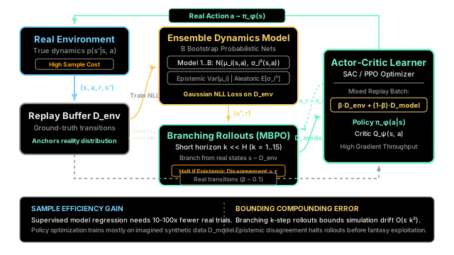
Why Does This Exist?

In standard model-free deep reinforcement learning (such as Soft Actor-Critic or Proximal Policy Optimization), an agent treats the environment as an opaque black box. To master a continuous control task, it typically requires millions of physical environment interactions. For real-world systems—such as industrial robotics, autonomous driving, or chemical manufacturing—collecting millions of trial-and-error interactions causes mechanical wear, consumes prohibitive operational time, and introduces catastrophic safety risks.

Model-free RL discards structural dynamics information: when an agent experiences a transition $(s_t, a_t, r_t, s_{t+1})$, it uses the sample exclusively to update a scalar value estimate or policy gradient. It completely ignores that the next state $s_{t+1}$ and reward $r_t$ are deterministic or stochastic functions of $(s_t, a_t)$.

Model-Based Deep RL bridges this sample-efficiency gap. By leveraging expressive deep neural networks as universal function approximators, the agent casts environment dynamics learning into a supervised regression problem. Because supervised neural networks learn orders of magnitude faster than trial-and-error RL, the agent quickly builds an accurate internal simulator. It can then generate millions of "imagined" synthetic rollouts entirely inside GPU memory, dramatically cutting physical sample complexity by $10\times$ to $100\times$.

Think of It Like This

How It Actually Works

The Core Dynamics Formulation and Model Exploitation

A Markov Decision Process (MDP) is defined by the tuple $(\mathcal{S}, \mathcal{A}, p, r, \gamma)$, where $p(s_{t+1} \mid s_t, a_t)$ represents the true environment transition distribution and $r(s_t, a_t)$ is the reward function.

In Model-Based Deep RL, the agent collects real transitions $\mathcal{D}_{\text{env}} = \{(s_t, a_t, r_t, s_{t+1})\}$ and trains parameterized neural networks to approximate the transition dynamics $\hat{p}_\theta(s_{t+1} \mid s_t, a_t)$ and reward function $\hat{r}_\psi(s_t, a_t)$.

To handle non-stationary and noisy physical systems, the transition model outputs a parameterized Gaussian distribution predicting state differences $\Delta s_t = s_{t+1} - s_t$:

$\hat{p}_\theta(s_{t+1} \mid s_t, a_t) = \mathcal{N}\left(s_t + \mu_\theta(s_t, a_t),\, \Sigma_\theta(s_t, a_t)\right)$

where $\mu_\theta(s_t, a_t)$ is the predicted mean change and $\Sigma_\theta(s_t, a_t) = \text{diag}(\sigma_\theta^2(s_t, a_t))$ models heteroscedastic aleatoric noise. The network parameters $\theta$ are trained by minimizing the Gaussian Negative Log-Likelihood (NLL) loss:

$\mathcal{L}_{\text{NLL}}(\theta) = \frac{1}{|\mathcal{D}_{\text{env}}|} \sum_{(s_t, a_t, s_{t+1}) \in \mathcal{D}_{\text{env}}} \left[ \frac{1}{2}\sum_{d=1}^D \left( \frac{(s_{t+1, d} - \hat{s}_{t+1, d})^2}{\sigma_{\theta, d}^2(s_t, a_t)} + \log \sigma_{\theta, d}^2(s_t, a_t) \right) \right]$

The Model Exploitation Problem

The core obstacle in naive model-based deep RL is model exploitation. When an off-policy actor-critic algorithm (such as SAC) is trained inside a single learned neural simulator $\hat{p}_\theta$, policy optimization relentlessly seeks actions that maximize predicted cumulative return.

Because deep neural networks are unconstrained outside their training distribution, the model makes arbitrary, inaccurate predictions in unvisited regions of the state-action space. If the neural network inadvertently predicts an artificially massive reward or an unphysical stable state, the policy optimizer locks onto this hallucinated loophole. When deployed in the real environment, the policy fails catastrophically because the hallucinated physics do not exist.

Uncertainty Quantification via Probabilistic Bootstrap Ensembles

To resolve model exploitation, algorithms such as PETS (Chua et al.) and MBPO (Janner et al.) employ a Probabilistic Bootstrap Ensemble of $B$ independent neural networks:

$\{\hat{p}_{\theta_1}, \hat{p}_{\theta_2}, \dots, \hat{p}_{\theta_B}\}$

Each ensemble member is initialized with different random weights and trained on randomly bootstrapped subsets of $\mathcal{D}_{\text{env}}$. This architecture cleanly isolates two distinct forms of uncertainty:

1. Aleatoric Uncertainty (Data Noise): The irreducible stochasticity inherent to the environment (e.g., sensor noise, friction variations). It is measured by the average predicted variance across ensemble members:

   $\bar{\sigma}^2(s_t, a_t) = \frac{1}{B} \sum_{i=1}^B \sigma_{\theta_i}^2(s_t, a_t)$

2. Epistemic Uncertainty (Model Ignorance): The uncertainty stemming from a lack of training data in that region of state space. It is quantified by the variance (disagreement) among the ensemble members' predicted means:

   $\text{Var}_{\text{epistemic}}(s_t, a_t) = \frac{1}{B} \sum_{i=1}^B \left(\mu_{\theta_i}(s_t, a_t) - \bar{\mu}(s_t, a_t)\right)^2, \quad \text{where } \bar{\mu}(s_t, a_t) = \frac{1}{B} \sum_{i=1}^B \mu_{\theta_i}(s_t, a_t)$

When an imagined rollout ventures into unfamiliar territory, epistemic disagreement spikes dramatically. The agent detects this divergence and either penalizes the reward with an epistemic penalty ($\tilde{r} = \hat{r} - \lambda \cdot \text{Var}_{\text{epistemic}}$) or immediately truncates the rollout.

Short-Horizon Branching Rollouts (MBPO)

Generating long imagined rollouts ($H = 1000$ steps) from an initial state $s_0$ causes simulation errors to compound quadratically:

$\text{Error}(k) \sim \mathcal{O}(\epsilon_{\text{model}} \cdot k^2)$

Model-Based Policy Optimization (MBPO) solves this by using short-horizon branching rollouts:

1. Uniformly sample a real state from the physical buffer: $s_0 \sim \mathcal{D}_{\text{env}}$.

2. Roll out the current policy $\pi_\phi$ using the ensemble dynamics model for only $k$ steps ($k \ll H$, typically $k \in [1, 15]$).

3. Store the generated synthetic transitions in a separate model buffer $\mathcal{D}_{\text{model}}$.

4. Train standard model-free Actor-Critic networks (SAC / PPO) on a mixed mini-batch:

   $\text{Batch} \sim \beta \mathcal{D}_{\text{env}} + (1 - \beta) \mathcal{D}_{\text{model}}, \quad \text{with } \beta \approx 0.05 \text{ to } 0.10$

Because rollouts are continually re-anchored to real states $s \in \mathcal{D}_{\text{env}}$ and restricted to a small horizon $k$, errors cannot compound runaway drift, yielding stable policy improvements.

Latent Dynamics and World Models

For visual domains (e.g., Atari, pixel-based manipulation), predicting raw pixels is computationally prohibitive and prone to blurring. Advanced model-based architectures—such as PlaNet (Hafner et al.) and Dreamer (Hafner et al.)—train a world model in a compact latent space:

• An encoder maps high-dimensional observations to latent states: $z_t = \text{enc}(o_t)$.
• A Recurrent State-Space Model (RSSM) predicts deterministic recurrent features $h_t$ and stochastic latent transitions $z_t \sim p(z_t \mid h_t)$.
• Policy optimization and value estimation are carried out purely within latent space rollouts, allowing million-step imagined rollouts with zero pixel decoding overhead during planning.

Worked numerical example

Consider an ensemble of $B = 3$ probabilistic dynamics models predicting the next state $s'$ given current state $s = 1.0$ and action $a = 0.5$.

Each ensemble member outputs its predicted mean $\mu_i$ and aleatoric variance $\sigma_i^2$:

• Model 1: $\mu_1 = 1.48$, $\sigma_1^2 = 0.010$
• Model 2: $\mu_2 = 1.52$, $\sigma_2^2 = 0.020$
• Model 3: $\mu_3 = 1.50$, $\sigma_3^2 = 0.015$

Step 1: Compute the Ensemble Predictive Mean

$\bar{\mu} = \frac{1}{3} (1.48 + 1.52 + 1.50) = \frac{4.50}{3} = 1.5000$

Step 2: Compute Aleatoric Uncertainty

$\bar{\sigma}^2 = \frac{1}{3} (0.010 + 0.020 + 0.015) = \frac{0.045}{3} = 0.015000$

Step 3: Compute Epistemic Uncertainty (Model Disagreement)

$\text{Var}_{\text{epistemic}} = \frac{1}{3} \sum_{i=1}^3 (\mu_i - \bar{\mu})^2$

$\text{Var}_{\text{epistemic}} = \frac{1}{3} \left( (1.48 - 1.50)^2 + (1.52 - 1.50)^2 + (1.50 - 1.50)^2 \right)$

$\text{Var}_{\text{epistemic}} = \frac{1}{3} \left( (-0.02)^2 + (0.02)^2 + 0.00^2 \right) = \frac{1}{3} (0.0004 + 0.0004 + 0.0000) = \frac{0.0008}{3} \approx 0.000267$

Step 4: Compute Total Predictive Variance

Applying the Law of Total Variance:

$\text{Var}_{\text{total}} = \bar{\sigma}^2 + \text{Var}_{\text{epistemic}} = 0.015000 + 0.000267 = 0.015267$

Step 5: Rollout Evaluation

The epistemic variance ($0.000267$) is well below the safety gating threshold $\tau = 0.05$. This indicates the transition lies firmly within the model's training distribution. The agent accepts the synthetic transition $(s=1.0, a=0.5, \hat{s}'=1.50)$ into $\mathcal{D}_{\text{model}}$ and proceeds to the next simulation step.

If the agent were instead to query an out-of-distribution state $s_{\text{OOD}} = 9.0$ where the models predict $\mu_1 = 8.1$, $\mu_2 = 11.4$, $\mu_3 = 6.0$, the epistemic variance would spike to $\approx 4.94 \gg \tau$, instantly halting the imagined branch before policy corruption occurs.

Code

Here is a complete, self-contained Python implementation of a Probabilistic Ensemble Dynamics Model supporting aleatoric/epistemic uncertainty decomposition and short-horizon branched rollouts with epistemic gating:

1from dataclasses import dataclass2from typing import List, Tuple3
4
5@dataclass6class Transition:7    step: int8    state: float9    action: float10    reward: float11    next_state: float12    epistemic_var: float13
14
15class ProbabilisticNet:16    """Simulated neural network member predicting continuous state delta and aleatoric variance."""17
18    def __init__(self, weight: float, bias: float, aleatoric_noise: float) -> None:19        self.weight = weight20        self.bias = bias21        self.noise = aleatoric_noise22
23    def forward(self, state: float, action: float) -> Tuple[float, float]:24        # Linear layer with action coupling: delta = w*s + 0.4*a + b25        delta_mean = self.weight * state + 0.4 * action + self.bias26        pred_next_state = state + delta_mean27        return pred_next_state, self.noise28
29
30class EnsembleDynamicsModel:31    """Bootstrap Ensemble of deep probabilistic models (PETS / MBPO style)."""32
33    def __init__(self, ensemble: List[ProbabilisticNet]) -> None:34        self.models = ensemble35        self.b = len(ensemble)36
37    def predict(38        self, state: float, action: float39    ) -> Tuple[float, float, float, float]:40        """Calculates ensemble predictive mean, aleatoric variance, epistemic variance,41
42        and total variance using the Law of Total Variance.43        """44        preds = [m.forward(state, action) for m in self.models]45        means = [p[0] for p in preds]46        variances = [p[1] for p in preds]47
48        # 1. Total predictive mean: bar_mu = (1/B) * sum(mu_i)49        bar_mu = sum(means) / self.b50
51        # 2. Aleatoric uncertainty: expected data variance52        bar_sigma2 = sum(variances) / self.b53
54        # 3. Epistemic uncertainty: model disagreement variance55        epistemic = sum((m - bar_mu) ** 2 for m in means) / self.b56
57        # 4. Total predictive variance58        total_var = bar_sigma2 + epistemic59
60        return bar_mu, bar_sigma2, epistemic, total_var61
62    def branch_rollout(63        self,64        seed_state: float,65        horizon_k: int,66        epistemic_gate: float,67    ) -> List[Transition]:68        """Rolls out synthetic transitions branching from a real replay buffer state.69
70        Truncates the rollout early if epistemic uncertainty exceeds the safety gate.71        """72        trajectory: List[Transition] = []73        curr_s = seed_state74
75        for step in range(1, horizon_k + 1):76            # Target policy action: negative feedback control a = -0.4 * s77            action = -0.4 * curr_s78
79            # Predict dynamics distribution80            next_s, aleatoric, epistemic, _ = self.predict(curr_s, action)81
82            # Quadratic cost reward: r = -(s^2 + 0.1 * a^2)83            reward = -(curr_s**2 + 0.1 * (action**2))84
85            # Epistemic truncation check86            if epistemic > epistemic_gate:87                print(88                    f"Step {step}: Epistemic gate triggered ({epistemic:.6f} > {epistemic_gate}). "89                    f"Truncating imagined rollout."90                )91                break92
93            trajectory.append(94                Transition(step, curr_s, action, reward, next_s, epistemic)95            )96            curr_s = next_s97
98        return trajectory99
100
101if __name__ == "__main__":102    # Initialize ensemble with B=3 calibrated probabilistic models103    net1 = ProbabilisticNet(weight=0.08, bias=0.20, aleatoric_noise=0.010)104    net2 = ProbabilisticNet(weight=0.12, bias=0.20, aleatoric_noise=0.020)105    net3 = ProbabilisticNet(weight=0.10, bias=0.20, aleatoric_noise=0.015)106
107    world_model = EnsembleDynamicsModel([net1, net2, net3])108
109    # 1. Evaluate single-step prediction (Numerical Worked Example)110    mu, aleatoric, epistemic, total = world_model.predict(state=1.0, action=0.5)111
112    print("=== Single Step Ensemble Prediction ===")113    print(f"Predictive Mean:      {mu:.4f}")114    print(f"Aleatoric Variance:   {aleatoric:.6f}")115    print(f"Epistemic Variance:   {epistemic:.6f}")116    print(f"Total Predictive Var: {total:.6f}")117
118    # Exact assertions matching worked numerical values119    assert abs(mu - 1.50) < 1e-6120    assert abs(aleatoric - 0.015) < 1e-6121    assert abs(epistemic - 0.0002667) < 1e-5122    assert abs(total - 0.0152667) < 1e-5123
124    # 2. Generate k=5 step branched rollout seeded from real state s=1.0125    print("\n=== Short-Horizon Branching Rollout (k=5) ===")126    synthetic_buffer = world_model.branch_rollout(127        seed_state=1.0, horizon_k=5, epistemic_gate=0.05128    )129    for t in synthetic_buffer:130        print(131            f"Step {t.step}: s={t.state:.3f}, a={t.action:.3f}, "132            f"r={t.reward:.3f}, s'={t.next_state:.3f}, epistemic={t.epistemic_var:.6f}"133        )

Expected output:

1=== Single Step Ensemble Prediction ===2Predictive Mean:      1.50003Aleatoric Variance:   0.0150004Epistemic Variance:   0.0002675Total Predictive Var: 0.0152676
7=== Short-Horizon Branching Rollout (k=5) ===8Step 1: s=1.000, a=-0.400, r=-1.016, s'=1.140, epistemic=0.0002679Step 2: s=1.140, a=-0.456, r=-1.320, s'=1.272, epistemic=0.00034710Step 3: s=1.272, a=-0.509, r=-1.643, s'=1.395, epistemic=0.00043111Step 4: s=1.395, a=-0.558, r=-1.978, s'=1.512, epistemic=0.00051912Step 5: s=1.512, a=-0.605, r=-2.321, s'=1.621, epistemic=0.000609

Watch Out For

The Quick Version

• Sample Efficiency via Supervised Learning: Model-Based Deep RL trains neural transition and reward models ($\hat{p}_\theta, \hat{r}_\psi$) using supervised regression, requiring $10\times$ to $100\times$ fewer real-world interactions than model-free algorithms.
• The Model Exploitation Threat: Policy optimizers exploit unconstrained out-of-distribution neural network errors, converging on hallucinated states where unrealistic rewards are predicted.
• Bootstrap Ensembles Quantify Uncertainty: Ensembles of $B$ deep probabilistic networks decouple irreducible aleatoric data noise from epistemic model ignorance ($\text{Var}_{\text{epistemic}}$), detecting when rollouts enter untrusted regions.
• Short-Horizon Branching (MBPO): Generating short rollouts ($k \ll H$, typically $k=1\dots15$) seeded from real replay buffer states $\mathcal{D}_{\text{env}}$ strictly bounds compounding simulation errors $\mathcal{O}(\epsilon k^2)$ while providing massive synthetic replay data for actor-critic optimization.

What to Read Next

• Learning Latent Dynamics
• Model-Based Policy Optimization (MBPO)
• Model-Based Reinforcement Learning