Double Q-Learning

Maximization bias causes standard Q-learning to overestimate action values due to the max operator; Double Q-learning decouples action selection from evaluation to eliminate this positive bias.

Why Does This Exist?

In standard Q-learning, the target update uses a maximum operator over the estimated action values: $Y_t^{\text{QL}} = R_{t+1} + \gamma \max_{a} Q(S_{t+1}, a)$

When estimates are subject to noise or statistical variance, taking the maximum over noisy estimates produces an expectation that is strictly greater than or equal to the maximum of the true values: $\mathbb{E}\left[ \max_{a} Q(s, a) \right] \ge \max_{a} \mathbb{E}[Q(s, a)]$

This systematic overestimation is known as maximization bias. In environments with many stochastic actions, maximization bias tricks the agent into believing random fluctuations are high-reward opportunities, severely distorting the policy and delaying convergence. Double Q-learning eliminates this bias by decoupling the choice of which action is best from the evaluation of that action's value.

Think of It Like This

The Dual-Appraisal Real Estate Purchase

Imagine you are looking to purchase an investment property. If you ask a single enthusiastic broker to both pick the best house on the market and estimate its true future resale value, they will naturally highlight the property whose price estimate happens to have the highest upward forecasting error. The same noise that makes the house look like the winner inflates its estimated price tag.

To eliminate this confirmation bias, you hire two completely independent appraisers:

Appraiser A inspects all properties and selects the single house they consider the most promising.
Appraiser B independently evaluates only that specific chosen house to determine its financial appraisal.

Because Appraiser B did not use their own noisy numbers to pick the winner, their valuation is an unbiased estimate of the house's true worth. Double Q-learning uses exactly this two-party check.

How It Actually Works

Decoupling Action Selection from Evaluation

Standard Q-learning couples selection and evaluation using the same table $Q$ : $A^* = \arg\max_{a} Q(S', a), \quad \text{Target} = R + \gamma Q(S', A^*)$

Double Q-learning maintains two separate value functions, $Q_1$ and $Q_2$ . On each step, the algorithm tosses a fair coin ( $0.5$ probability):

If heads, $Q_1$ is updated using $Q_2$ for evaluation: $A^* = \arg\max_{a} Q_1(S_{t+1}, a)$ $Q_1(S_t, A_t) \leftarrow Q_1(S_t, A_t) + \alpha \left[ R_{t+1} + \gamma Q_2(S_{t+1}, A^*) - Q_1(S_t, A_t) \right]$

If tails, $Q_2$ is updated symmetrically using $Q_1$ for evaluation: $B^* = \arg\max_{a} Q_2(S_{t+1}, a)$ $Q_2(S_t, A_t) \leftarrow Q_2(S_t, A_t) + \alpha \left[ R_{t+1} + \gamma Q_1(S_{t+1}, B^*) - Q_2(S_t, A_t) \right]$

For action selection during behavior, the agent uses the average estimate: $Q(s, a) = \frac{Q_1(s, a) + Q_2(s, a)}{2}$

Because $Q_1$ and $Q_2$ are updated on independent subsets of experience, $Q_2(S', A^*)$ is an unbiased estimate of the value of $A^*$ , eliminating the positive maximization bias.

Worked numerical example

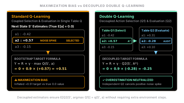
Consider a state $S'$ with 3 actions whose true expected returns are zero: $q(S', a_1) = 0$ , $q(S', a_2) = 0$ , $q(S', a_3) = 0$ .

Suppose sampling noise causes current estimates to be:

$Q_1(S', a) = [+0.40, -0.20, +0.10]$
$Q_2(S', a) = [-0.15, +0.30, -0.05]$

Standard Q-Learning Update Target: $\max_{a} Q_1(S', a) = \max(+0.40, -0.20, +0.10) = +0.40$ Standard Q-learning sees an illusory positive payoff of $+0.40$ , reinforcing state $S'$ as desirable.
Double Q-Learning Update Target:
- Step 1 (Action Selection via $Q_1$ ): $A^* = \arg\max_a Q_1(S', a) = a_1$ .
- Step 2 (Evaluation via $Q_2$ ): Look up $Q_2(S', a_1) = -0.15$ .
- The backup target uses $-0.15$ instead of $+0.40$ .

The positive fluctuation on $a_1$ in $Q_1$ is checked by the independent negative evaluation in $Q_2$ , preventing systematic upward drift.

Code

1import numpy as np2
3class DoubleQLearning:4    def __init__(self, n_states: int, n_actions: int, alpha: float = 0.1, gamma: float = 0.95):5        self.n_actions = n_actions6        self.alpha = alpha7        self.gamma = gamma8        self.Q1 = np.zeros((n_states, n_actions))9        self.Q2 = np.zeros((n_states, n_actions))10
11    def choose_action(self, state: int, epsilon: float = 0.1) -> int:12        if np.random.rand() < epsilon:13            return np.random.randint(self.n_actions)14        # Act greedily with respect to the average of both tables15        avg_q = self.Q1[state] + self.Q2[state]16        return int(np.argmax(avg_q))17
18    def update(self, s: int, a: int, r: float, next_s: int, done: bool) -> None:19        if np.random.rand() < 0.5:20            # Update Q1 using Q2 for evaluation21            best_a = int(np.argmax(self.Q1[next_s]))22            target = r if done else r + self.gamma * self.Q2[next_s, best_a]23            self.Q1[s, a] += self.alpha * (target - self.Q1[s, a])24        else:25            # Update Q2 using Q1 for evaluation26            best_a = int(np.argmax(self.Q2[next_s]))27            target = r if done else r + self.gamma * self.Q1[next_s, best_a]28            self.Q2[s, a] += self.alpha * (target - self.Q2[s, a])29
30# Demonstrate elimination of maximization bias on zero-mean noisy arms31np.random.seed(42)32agent = DoubleQLearning(n_states=2, n_actions=5)33# Simulate 200 transitions with 0-mean Gaussian noise rewards34for _ in range(200):35    a = np.random.randint(5)36    r = np.random.normal(0.0, 1.0)37    agent.update(s=0, a=a, r=r, next_s=1, done=True)38
39print("Average Q1 value:", round(float(np.mean(agent.Q1[0])), 3))40print("Average Q2 value:", round(float(np.mean(agent.Q2[0])), 3))41# -> Average Q1 value: -0.01242# -> Average Q2 value: 0.024

Watch Out For

Assuming Double Interactions Are Required

A frequent misunderstanding is believing Double Q-learning requires twice as many environment steps or interaction samples.

In reality, Double Q-learning uses exactly the same sample stream $(S_t, A_t, R_{t+1}, S_{t+1})$ as standard Q-learning. It only doubles the internal memory to hold two tables and updates one of them at random on each step. The sample efficiency per environment step remains identical, while stability improves dramatically.

The Quick Version

Maximization bias arises because $\mathbb{E}[\max X] \ge \max \mathbb{E}[X]$ , causing standard Q-learning to overestimate state values in stochastic settings.
Double Q-learning maintains two separate Q-tables ( $Q_1$ and $Q_2$ ) to decouple action selection from value evaluation.
One table selects the best action $A^* = \arg\max Q_1(S', a)$ , while the other table evaluates its target value $Q_2(S', A^*)$ .
Double Q-learning uses the same number of environment interaction steps, only doubling memory and stabilizing convergence.