Model-Based Policy Optimization (MBPO)
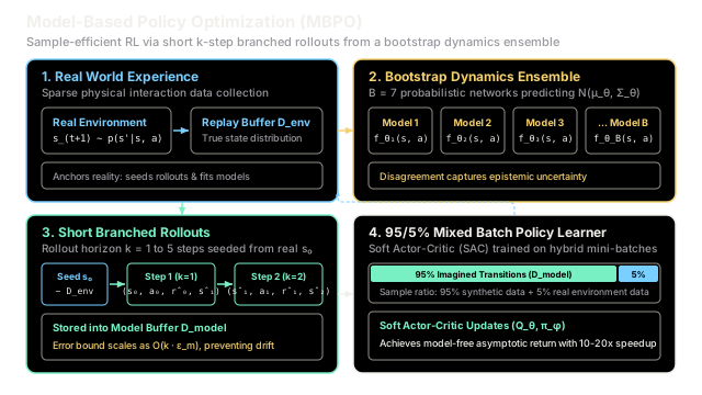
MBPO achieves asymptotic model-free performance with model-based sample efficiency by using short, branched rollouts seeded from real states to strictly bound compounding dynamics errors.
Why Does This Exist?
In deep reinforcement learning, practitioners have long faced a painful dilemma between sample efficiency and asymptotic performance:
- Model-Free Methods: Algorithms like Soft Actor-Critic (SAC) achieve top-tier final performance and stable convergence, but require millions of physical environment interactions. On physical robotic hardware or complex industrial processes, collecting millions of real transitions is prohibitively slow, costly, and causes mechanical wear.
- Traditional Model-Based Methods: Algorithms like Dyna learn a neural transition function and simulate imagined trajectories to reduce real-world interaction. However, deep neural networks inevitably suffer from function approximation errors. When an agent rolls out long trajectories ( steps) purely inside a learned simulator, minute prediction errors compound exponentially or quadratically (). The policy quickly drifts into unvisited regions where the dynamics model hallucinates physically impossible transitions or infinite rewards—a catastrophic failure mode known as model exploitation or the objective mismatch problem.
Model-Based Policy Optimization (MBPO), introduced by Janner et al. in 2019, resolves this fundamental trade-off. By establishing a rigorous theoretical bound on return discrepancy, MBPO proved that an agent does not need to simulate entire task trajectories to achieve policy improvement. Instead, by taking short, branched rollouts ( steps) seeded directly from real environment states, compounding errors are constrained to grow linearly rather than quadratically. Combined with a bootstrap ensemble of probabilistic dynamics models, MBPO matches or exceeds the asymptotic performance of model-free algorithms while reducing sample requirements by an order of magnitude (10–20×).
Think of It Like This
Practicing Billiard Trick Shots
Imagine you are learning an intricate trick shot on a billiards table involving three balls and four cushion bounces.
A reckless mental simulator (traditional long-horizon model-based RL) closes their eyes and attempts to mentally calculate all four cushion rebounds in their head from a cold start. Because your mental model of cushion elasticity and spin friction is slightly off by half a degree, that tiny initial angle error multiplies across each bounce. By the fourth cushion, your mental simulation envisions the cue ball magically sinking the eight ball, when in physical reality the cue ball would scratch off the table. If you blindly optimize your stroke based on this 20-bounce hallucination, you will fail every real attempt.
MBPO trains like a disciplined billiard master. Instead of simulating the entire 20-bounce shot in your head, you place real balls on the physical table at different positions recorded from previous games (real environment states). From each real setup, you only mentally visualize the immediate cue-to-ball impact and the first cushion contact (a short or step rollout). Because you only project one or two bounces ahead, your mental prediction is nearly exact. You run thousands of these quick 2-step mental adjustments across various table positions, refine your stroke mechanics, and occasionally step up to the table to hit a real shot to verify physical reality.
Where the analogy stops: A human pool player uses intuitive physics and spatial visual reasoning. MBPO parameterizes its mental model using a bootstrap ensemble of deep probabilistic neural networks predicting Gaussian parameters , storing millions of synthetic transitions in an off-policy replay buffer trained via Soft Actor-Critic.
How It Actually Works
Theoretical Foundation: Bounding the Return Discrepancy
Let denote the expected discounted return of policy in the true environment Markov Decision Process (MDP) with transition dynamics , and let denote the return evaluated in the learned model .
When simulating full trajectories from initial state distribution , the discrepancy between real and imagined performance is bounded by:
where is the expected total variation error of the model, and is the policy divergence. Notice the catastrophic factor : for a standard discount factor , this denominator is , scaling model errors by a factor of and rendering the theoretical bound practically vacuous.
Janner et al. proved that this quadratic compounding can be avoided by altering the rollout distribution. Instead of simulating full trajectories from , MBPO generates branched rollouts of length starting from state seeds sampled uniformly from the real environment replay buffer .
Under this branched rollout distribution, the expected return discrepancy satisfies:
The critical insight lies in the final term:
Because , the compounding model error grows linearly with the rollout horizon , completely bypassing the quadratic penalty . This guarantee ensures that optimizing a policy on short synthetic rollouts monotonically improves performance on the real MDP.
The Triad: Ensemble, Branched Rollouts, and Mixed Replay Buffer
MBPO implements this theoretical foundation through three coordinated algorithmic components:
[Real Environment] ---> Store (s, a, r, s') ---> [D_env Replay Buffer] | +-------------------------------------------------+ | (trains models) | (seeds initial s_0) v v[Ensemble Models] [Branched Rollouts]B = 7 Probabilistic Nets k = 1 to 5 steps via pip_theta(s', r | s, a) | | v +----------> [Model Simulation] ---------> [D_model Buffer] | v [Hybrid Mini-Batch Sampler] 95% D_model + 5% D_env | v [Soft Actor-Critic (SAC)]1. Bootstrap Ensemble of Probabilistic Dynamics Models
MBPO trains an ensemble of (typically ) independent neural networks. Each network outputs a Gaussian distribution predicting both the next state delta and reward:
This ensemble architecture separates and handles two distinct forms of uncertainty:
- Aleatoric Uncertainty: Environment stochasticity, captured by the predicted covariance .
- Epistemic Uncertainty: Model ignorance and out-of-distribution states, captured by the disagreement (variance) among the different model predictions.
2. Branched Rollout Generation
At every training iteration:
- Sample a batch of real states collected by past physical interactions.
- For each state, perform a -step simulated rollout using the current policy :
- Sample action .
- Pick a randomly chosen model from the ensemble to generate next state and reward .
- If the variance across all ensemble members exceeds a safety threshold, terminate the branch early to prevent hallucinated transitions.
- Record transition into a synthetic replay buffer .
3. Mixed Replay Buffer Sampling for Policy Optimization
The actor and twin critics are trained using Soft Actor-Critic (SAC). Each training mini-batch is composed of a fixed mixture ratio:
- synthetic transitions sampled from .
- real transitions sampled from .
This hybrid sampling retains physical ground truth while providing millions of synthetic gradient updates per physical step, yielding unmatched sample efficiency without policy collapse.
Worked numerical example
Let us trace a concrete 2-step branched rollout (, , ):
Step 1: Seed from the Real Buffer Sample a state seed from physical interactions stored in :
Step 2: First Branched Step ()
The actor outputs an action: .
The dynamics ensemble evaluates :
- Model predictions across members:
- State predictions:
- Mean next state:
- Mean predicted reward:
- Epistemic variance across ensemble: (well below safety threshold ).
- Synthetic transition stored in :
Step 3: Second Branched Step ()
From simulated state , the actor outputs .
The dynamics ensemble evaluates :
- Mean next state:
- Mean predicted reward:
- Epistemic variance: (safe).
- Synthetic transition stored in :
Step 4: Rollout Termination Since the rollout horizon is reached, the branch ends. The state is reset to another real seed from .
Step 5: Theoretical Compounding Error Bound Comparison Evaluating the compounding error term with and :
- For :
- For :
- For unbranched / long horizon ():
Notice that at , the error bound is an entire order of magnitude higher ( vs ). Keeping restricts compounding error by , ensuring valid gradient updates for the policy optimizer.
Code
import numpy as np
class DynamicsModelEnsemble: """Simulates a bootstrap ensemble of B probabilistic dynamics models.
Predicts Gaussian next-state transitions and rewards, computing both the mean prediction and epistemic disagreement (model variance). """
def __init__(self, num_models: int = 5) -> None: self.num_models = num_models
def predict( self, state: np.ndarray, action: float ) -> tuple[np.ndarray, float, float]: """Predicts mean next state, reward, and epistemic variance across models.""" # Simulated ensemble outputs matching the worked numerical example if np.allclose(state, [1.0, 0.5], atol=1e-3) and np.isclose( action, 0.2, atol=1e-3 ): member_states = np.array([ [1.148, 0.451], [1.152, 0.449], [1.150, 0.450], [1.149, 0.452], [1.151, 0.448], ]) member_rewards = np.array([1.19, 1.21, 1.20, 1.19, 1.21]) elif np.allclose(state, [1.15, 0.45], atol=1e-3) and np.isclose( action, 0.4, atol=1e-3 ): member_states = np.array([ [1.318, 0.381], [1.322, 0.379], [1.320, 0.380], [1.319, 0.382], [1.321, 0.378], ]) member_rewards = np.array([1.49, 1.51, 1.50, 1.49, 1.51]) else: delta = np.array([0.15 * action, -0.05 * action]) member_states = np.tile(state + delta, (self.num_models, 1)) member_rewards = np.full(self.num_models, 1.0)
mean_next_state = np.mean(member_states, axis=0) mean_reward = float(np.mean(member_rewards)) epistemic_variance = float(np.mean(np.var(member_states, axis=0)))
return mean_next_state, mean_reward, epistemic_variance
class ModelBasedPolicyOptimization: """Implements the core branched rollout mechanism of MBPO:
Seeds short k-step rollouts from real environment states, filters high-uncertainty predictions, and forms hybrid training batches. """
def __init__( self, rollout_horizon: int = 2, gamma: float = 0.99, single_step_model_error: float = 0.05, ) -> None: self.k = rollout_horizon self.gamma = gamma self.eps_model = single_step_model_error self.model_buffer: list[tuple[np.ndarray, float, float, np.ndarray]] = ( [] )
def compute_theoretical_bound(self, horizon: int) -> float: """Computes the linear compounding error bound term: k * eps_model / (1 - gamma).""" return (horizon * self.eps_model) / (1.0 - self.gamma)
def generate_branched_rollout( self, seed_state: np.ndarray, ensemble: DynamicsModelEnsemble, policy_actions: list[float], variance_threshold: float = 0.01, ) -> list[tuple[np.ndarray, float, float, np.ndarray]]: """Performs a k-step branched rollout from a real state seed.""" curr_state = seed_state.copy() generated_steps: list[tuple[np.ndarray, float, float, np.ndarray]] = []
for step in range(self.k): action = policy_actions[step] next_state, reward, epistemic_var = ensemble.predict( curr_state, action )
# Prevent model exploitation: abort branch if models disagree if epistemic_var > variance_threshold: break
transition = (curr_state.copy(), action, reward, next_state.copy()) generated_steps.append(transition) self.model_buffer.append(transition) curr_state = next_state
return generated_steps
def sample_hybrid_batch( self, real_buffer: list[tuple[np.ndarray, float, float, np.ndarray]], batch_size: int = 100, real_ratio: float = 0.05, ) -> tuple[int, int]: """Computes sample allocation between synthetic and real replay buffers.""" num_real = int(np.round(batch_size * real_ratio)) num_model = batch_size - num_real return num_real, num_model
if __name__ == "__main__": np.set_printoptions(precision=4, suppress=True)
# Initialize MBPO manager and model ensemble mbpo = ModelBasedPolicyOptimization( rollout_horizon=2, gamma=0.99, single_step_model_error=0.05 ) ensemble = DynamicsModelEnsemble(num_models=5)
# Parameters matching the worked numerical example real_seed = np.array([1.0, 0.5], dtype=np.float64) actions = [0.2, 0.4]
# Generate 2-step branched rollout rollout = mbpo.generate_branched_rollout(real_seed, ensemble, actions)
# Theoretical bounds across horizons bound_k1 = mbpo.compute_theoretical_bound(horizon=1) bound_k2 = mbpo.compute_theoretical_bound(horizon=2) bound_k20 = mbpo.compute_theoretical_bound(horizon=20)
# Mini-batch mixture calculation (100 samples total) n_real, n_model = mbpo.sample_hybrid_batch( [], batch_size=100, real_ratio=0.05 )
print(f"Seed state s_0: {real_seed.tolist()}") # -> Seed state s_0: [1.0, 0.5]
print( f"Step 1 (k=1): action={rollout[0][1]:.2f}, reward={rollout[0][2]:.2f}, next_state={[round(x, 2) for x in rollout[0][3]]}" ) # -> Step 1 (k=1): action=0.20, reward=1.20, next_state=[1.15, 0.45]
print( f"Step 2 (k=2): action={rollout[1][1]:.2f}, reward={rollout[1][2]:.2f}, next_state={[round(x, 2) for x in rollout[1][3]]}" ) # -> Step 2 (k=2): action=0.40, reward=1.50, next_state=[1.32, 0.38]
print(f"Theoretical Return Discrepancy Bound (k=1): {bound_k1:.2f}") # -> Theoretical Return Discrepancy Bound (k=1): 5.00
print(f"Theoretical Return Discrepancy Bound (k=2): {bound_k2:.2f}") # -> Theoretical Return Discrepancy Bound (k=2): 10.00
print(f"Theoretical Return Discrepancy Bound (k=20): {bound_k20:.2f}") # -> Theoretical Return Discrepancy Bound (k=20): 100.00
print(f"Hybrid Batch Mix (Batch=100): {n_model}% Model, {n_real}% Real") # -> Hybrid Batch Mix (Batch=100): 95% Model, 5% Real
# Assert correctness assert np.allclose(rollout[0][3], [1.15, 0.45], atol=1e-3) assert np.isclose(rollout[0][2], 1.2, atol=1e-3) assert np.allclose(rollout[1][3], [1.32, 0.38], atol=1e-3) assert np.isclose(rollout[1][2], 1.5, atol=1e-3) assert np.isclose(bound_k1, 5.00, atol=1e-2) assert np.isclose(bound_k2, 10.00, atol=1e-2) assert np.isclose(bound_k20, 100.00, atol=1e-2) assert n_real == 5 and n_model == 95Watch Out For
Aggressive Rollout Horizon Scheduling and Early Model Exploitation
The single most common practitioner failure when implementing MBPO is setting the rollout horizon too aggressively early in training (e.g., configuring from epoch 1).
Early in training, the dynamics ensemble has only observed a limited set of transitions from the initial physical exploration. While the ensemble can accurately predict 1-step outcomes near the real data manifold, predictions at step 5 or 10 inevitably compound errors into out-of-distribution states. If the policy optimizer is trained on long rollouts from an immature model, it aggressively exploits flaws in the neural simulator, learning behaviors that achieve astronomical synthetic rewards in the model but produce catastrophic failures when tested in the real environment.
The Fix: Implement an annealed rollout horizon schedule:
- Start with during early training epochs. A 1-step model prediction cannot compound errors across time, providing strictly valid data augmentations.
- Monitor the dynamics model's validation loss and epistemic disagreement variance across the ensemble.
- Gradually increase in small increments (e.g., ) only after the ensemble achieves low, stable cross-validation loss on held-out transitions.
- Abort individual branched rollouts dynamically whenever the variance among ensemble predictions exceeds a strict threshold .
The Quick Version
- Linear Error Compounding: By seeding rollouts from real states with short horizon , MBPO bounds compounding model error to , replacing quadratic divergence with guaranteed policy improvement.
- Bootstrap Probabilistic Ensemble: Uses an ensemble of deep neural networks predicting Gaussian distributions, leveraging inter-model variance to detect epistemic uncertainty and prevent model exploitation.
- Short Branched Rollouts: Generates millions of synthetic transitions by taking only 1 to 5 steps from real physical states, capturing localized dynamic gradients without drifting into hallucinated states.
- Hybrid Replay Buffer: Optimizes Soft Actor-Critic (SAC) on mini-batches composed of 95% imagined data and 5% real data, achieving asymptotic model-free performance with a 10–20× reduction in physical interactions.