MuZero and AlphaZero

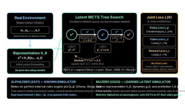
Why Does This Exist?

In 2017, DeepMind introduced AlphaZero, achieving superhuman mastery across Chess, Shogi, and Go using a tabula rasa combination of deep neural networks and Monte Carlo Tree Search (MCTS). However, AlphaZero suffered from a critical limitation: it relied on a perfect, handcrafted, external simulator $p(s' \mid s, a)$. At every node expansion in the search tree, the algorithm asked the ground-truth game engine: "If I play move $a$ from board $s$, what is the exact legal next board state $s'$?"

In real-world reinforcement learning—such as robotics, autonomous vehicles, visual video games, or financial forecasting—a perfect forward simulator does not exist. The dynamics are complex, noisy, or unknown.

Early model-based reinforcement learning methods attempted to overcome this by building world models that reconstructed raw observations (e.g., predicting future video frames pixel-by-pixel). This proved inefficient and fragile: neural networks wasted vast capacity trying to reproduce visually intricate but task-irrelevant details (such as fluttering leaves or flickering background score counters) while suffering from compounding prediction drift.

MuZero (Schrittwieser et al., 2020) resolved this bottleneck with a fundamental conceptual breakthrough: an agent does not need to reconstruct the world to plan effectively—it only needs to model what directly impacts its decisions. Instead of predicting raw observation transitions, MuZero trains deep neural networks to predict only three decision-critical quantities: the policy $\mathbf{p}$, the value $v$, and the immediate reward $r$. By executing MCTS purely inside an abstract, learned latent state space, MuZero matched AlphaZero in Chess and Go while simultaneously setting state-of-the-art benchmark records across visually rich Atari 2600 games without ever knowing the rules of the environment.

Think of It Like This

How It Actually Works

From AlphaZero to MuZero: The Simulator Bottleneck

AlphaZero combines a dual-head deep neural network $f_\theta(s) = (\mathbf{p}, v)$ with Monte Carlo Tree Search. During MCTS, nodes represent ground-truth environment states $s$, and directed edges represent actions $a$.

At each state $s$, actions are selected using the Predictor Upper Confidence Bound applied to Trees (PUCT) formula:

$a_t = \arg\max_a \left[ Q(s, a) + c_{\text{puct}} \cdot P(s, a) \cdot \frac{\sqrt{\sum_b N(s, b)}}{1 + N(s, a)} \right]$

where:

• $Q(s, a)$ is the running mean action-value of the edge.
• $P(s, a)$ is the prior probability of selecting action $a$, supplied by the policy head of $f_\theta(s)$.
• $N(s, a)$ is the number of times action $a$ has been traversed from node $s$.
• $\sum_b N(s, b)$ is the total visit count of parent state $s$.
• $c_{\text{puct}}$ is an exploration parameter balancing exploitation of high-$Q$ branches against exploration of low-visit branches.

Once a leaf node is reached, AlphaZero invokes the exact environment rules engine: $s' = \text{env}.\text{step}(s, a)$ to instantiate the child state, evaluates $s'$ using $f_\theta(s')$, and backs up the predicted value $v$ along the search path.

The MuZero Triplet: Representation, Dynamics, and Prediction

MuZero removes the environment simulator by parameterizing the world model through three neural network functions:

1Observation History (o₁...o_t)2        │3        ▼4┌───────────────────────────────┐5│ Representation Function h_θ   │  ──>  s⁰ (Initial Latent State)6└───────────────────────────────┘7        │8        ├──────────────────────────────────────┐9        ▼                                      ▼10┌───────────────────────────────┐      ┌───────────────────────────────┐11│ Dynamics Function g_θ         │      │ Prediction Function f_θ       │12│ (s^{k-1}, a^k) ──> (r^k, s^k) │      │ s^k ──> (p^k, v^k)            │13└───────────────────────────────┘      └───────────────────────────────┘

1. Representation Function ($h_\theta$): $s^0 = h_\theta(o_1, o_2, \dots, o_t)$ Encodes the historical sequence of past observations into an initial abstract hidden state $s^0$. In visual Atari tasks, $h_\theta$ is a convolutional network (CNN) or ResNet processing stacked image frames.

2. Dynamics Function ($g_\theta$): $(r^k, s^k) = g_\theta(s^{k-1}, a^k)$ Acts as the internal, learned simulator. Given the previous hidden state $s^{k-1}$ and candidate action $a^k$, it recurrently outputs the predicted next hidden state $s^k$ and the immediate scalar reward $r^k$. Note that $s^k$ does not have any semantic obligation to resemble a decoded image; it is purely an abstract computational substrate.

3. Prediction Function ($f_\theta$): $(\mathbf{p}^k, v^k) = f_\theta(s^k)$ Evaluates any hidden state $s^k$ generated during tree search, producing:

   • Policy distribution $\mathbf{p}^k$: a probability vector over all legal actions.
   • Value estimate $v^k$: the expected cumulative discounted future return from state $s^k$.

Latent MCTS: Planning Without Ground Truth

During inference and acting, MuZero runs MCTS entirely in hidden state space across four distinct phases:

1. Selection: Starting at root node $s^0$, the agent recursively traverses edges choosing action $a^k$ that maximizes the PUCT objective until reaching an unexpanded edge. To stabilize search across games with varied reward scales, MuZero normalizes $Q$-values into $[0, 1]$ using min-max tracking: $\bar{Q}(s, a) = \frac{Q(s, a) - Q_{\min}}{Q_{\max} - Q_{\min}}$
2. Expansion: The selected action $a^k$ and parent state $s^{k-1}$ are fed into the learned dynamics function: $(r^k, s^k) = g_\theta(s^{k-1}, a^k)$ creating a new child node with hidden state $s^k$ and edge reward $r^k$.
3. Evaluation: The newly created state $s^k$ is passed through the prediction network: $(\mathbf{p}^k, v^k) = f_\theta(s^k)$ storing prior probabilities $\mathbf{p}^k$ on outgoing edges.
4. Backup: The leaf value $v^k$ is discounted and propagated back up the search path. For a trajectory of depth $d$, the $m$-step return backed up to edge $(s^{m-1}, a^m)$ is: $G^m = \sum_{\tau=0}^{d-m-1} \gamma^\tau r^{m+\tau+1} + \gamma^{d-m} v^k$ Edge statistics are updated: $N(s^{m-1}, a^m) \leftarrow N(s^{m-1}, a^m) + 1$ $Q(s^{m-1}, a^m) \leftarrow \frac{N(s^{m-1}, a^m) \cdot Q(s^{m-1}, a^m) + G^m}{N(s^{m-1}, a^m) + 1}$

Once search concludes (e.g., after 50–800 simulations), an action $a_t$ is selected in the real environment proportionally to visit counts: $\pi_t(a) = \frac{N(s^0, a)^{1/T}}{\sum_b N(s^0, b)^{1/T}}$ where $T$ is a temperature parameter ($T=1$ for exploratory self-play, $T \to 0$ for competitive deployment).

End-to-End Joint Loss Without Observation Reconstruction

MuZero trains all three networks ($h_\theta, g_\theta, f_\theta$) end-to-end via gradient descent. Trajectories are sampled from a replay buffer, and the model is unrolled for $K$ hypothetical simulation steps ($K=5$ typically):

$\mathcal{L}(\theta) = \sum_{k=0}^K \left[ \ell_p(\pi_{t+k}, \mathbf{p}_t^k) + \ell_v(z_{t+k}, v_t^k) \right] + \sum_{k=1}^K \ell_r(u_{t+k}, r_t^k) + c \|\theta\|^2$

where:

• $\ell_p(\pi, \mathbf{p}) = -\sum \pi \log \mathbf{p}$ is the cross-entropy loss aligning the predicted policy with the MCTS visit distribution $\pi$.
• $\ell_v(z, v)$ is the loss between predicted value $v_t^k$ and target return $z_{t+k}$ (computed from bootstrapped $n$-step returns or final game outcomes).
• $\ell_r(u, r)$ is the loss matching predicted reward $r_t^k$ to real observed reward $u_{t+k}$.
• $c \|\theta\|^2$ is $L_2$ weight regularization.

Because gradients flow from $\ell_p, \ell_v,$ and $\ell_r$ backward through the dynamics function $g_\theta$ and representation function $h_\theta$, the hidden states are forced to capture all information necessary to predict value, policy, and rewards—and strictly nothing else.

Worked numerical example

Let us trace a concrete single-step MCTS iteration in latent state space ($k=1$) with exploration parameter $c_{\text{puct}} = 1.0$ and discount $\gamma = 0.9$.

Initial Root State Setup

• Initial root hidden state: $s^0 = [0.8, -0.4]$
• Root prediction: $f_\theta(s^0) \to \mathbf{p}^0 = \{a_1: 0.7,\, a_2: 0.3\}$, $v^0 = 1.5$
• Current tree edge visit counts:
  • $N(s^0, a_1) = 3$
  • $N(s^0, a_2) = 1$
  • Total parent visits: $\sum_b N(s^0, b) = 3 + 1 = 4$
• Current edge action-values:
  • $Q(s^0, a_1) = 1.2$
  • $Q(s^0, a_2) = 0.8$

Step 1: Compute PUCT Exploration Scores

For Action $a_1$: $U(s^0, a_1) = c_{\text{puct}} \cdot P(s^0, a_1) \cdot \frac{\sqrt{\sum_b N(s^0, b)}}{1 + N(s^0, a_1)} = 1.0 \times 0.7 \times \frac{\sqrt{4}}{1 + 3} = 0.7 \times \frac{2}{4} = 0.3500$ $\text{Score}(s^0, a_1) = Q(s^0, a_1) + U(s^0, a_1) = 1.2 + 0.3500 = 1.5500$

For Action $a_2$: $U(s^0, a_2) = c_{\text{puct}} \cdot P(s^0, a_2) \cdot \frac{\sqrt{\sum_b N(s^0, b)}}{1 + N(s^0, a_2)} = 1.0 \times 0.3 \times \frac{\sqrt{4}}{1 + 1} = 0.3 \times \frac{2}{2} = 0.3000$ $\text{Score}(s^0, a_2) = Q(s^0, a_2) + U(s^0, a_2) = 0.8 + 0.3000 = 1.1000$

Step 2: Action Selection

Comparing the candidate PUCT scores: $\text{Score}(s^0, a_1) = 1.5500 > 1.1000 = \text{Score}(s^0, a_2)$ The agent selects action $a_1$.

Step 3: Latent Dynamics Expansion

The agent passes $(s^0, a_1)$ into the learned dynamics function: $g_\theta(s^0, a_1) \longrightarrow s^1 = [0.9, -0.2], \quad r^1 = 0.5000$

Step 4: Latent Prediction Evaluation

The child hidden state $s^1$ is evaluated by the prediction network: $f_\theta(s^1) \longrightarrow \mathbf{p}^1 = \{a_1: 0.6,\, a_2: 0.4\}, \quad v^1 = 2.0000$

Step 5: Backpropagation Backup Update

The backup return for edge $(s^0, a_1)$ is computed using the immediate reward and discounted child value: $\text{Backup Return } G = r^1 + \gamma \cdot v^1 = 0.5 + 0.9 \times 2.0000 = 0.5 + 1.8000 = 2.3000$

Now update the statistics for edge $(s^0, a_1)$:

• Previous total value: $\text{Total Value}_{\text{old}} = N \times Q = 3 \times 1.2 = 3.6000$
• New visit count: $N_{\text{new}}(s^0, a_1) = 3 + 1 = 4$
• New total value: $\text{Total Value}_{\text{new}} = 3.6000 + 2.3000 = 5.9000$
• New updated $Q$-value: $Q_{\text{new}}(s^0, a_1) = \frac{\text{Total Value}_{\text{new}}}{N_{\text{new}}} = \frac{5.9000}{4} = 1.4750$

The edge action-value increases from $1.2000$ to $1.4750$, reflecting the promising simulated transition discovered in latent space.

Code

Below is a self-contained, type-hinted Python implementation of the core MuZero model architecture ($h_\theta, g_\theta, f_\theta$) and the latent MCTS node selection, expansion, and backpropagation backup:

1from dataclasses import dataclass, field2import math3from typing import Dict, List, Tuple4
5
6@dataclass7class MCTSNode:8    """Represents a node in MuZero's latent Monte Carlo search tree."""9
10    hidden_state: List[float]11    prior_p: float = 0.012    visit_count: int = 013    total_value: float = 0.014    reward: float = 0.015    children: Dict[str, "MCTSNode"] = field(default_factory=dict)16
17    @property18    def q_value(self) -> float:19        if self.visit_count == 0:20            return 0.021        return self.total_value / self.visit_count22
23
24class MuZeroModel:25    """MuZero's three parameterized neural functions operating on latent states."""26
27    def h_representation(self, observations: List[float]) -> List[float]:28        """s^0 = h_theta(o_1...o_t): Encodes observation history into initial latent state."""29        # Maps input observation directly to initial abstract hidden state30        return list(observations)31
32    def g_dynamics(33        self, hidden_state: List[float], action: str34    ) -> Tuple[List[float], float]:35        """(s^k, r^k) = g_theta(s^{k-1}, a^k): Recurrently predicts next hidden state and reward."""36        if action == "a_1":37            # Latent transition for action a_138            return [0.9, -0.2], 0.539        else:40            # Latent transition for action a_241            return [0.7, -0.6], 0.142
43    def f_prediction(44        self, hidden_state: List[float]45    ) -> Tuple[Dict[str, float], float]:46        """(p^k, v^k) = f_theta(s^k): Predicts policy probabilities and state value."""47        if math.isclose(hidden_state[0], 0.8) and math.isclose(48            hidden_state[1], -0.449        ):50            return {"a_1": 0.7, "a_2": 0.3}, 1.551        elif math.isclose(hidden_state[0], 0.9) and math.isclose(52            hidden_state[1], -0.253        ):54            return {"a_1": 0.6, "a_2": 0.4}, 2.055        else:56            return {"a_1": 0.5, "a_2": 0.5}, 1.057
58
59class LatentMCTS:60    """Monte Carlo Tree Search executed entirely within learned hidden state space."""61
62    def __init__(63        self,64        model: MuZeroModel,65        c_puct: float = 1.0,66        discount_gamma: float = 0.9,67    ) -> None:68        self.model = model69        self.c_puct = c_puct70        self.gamma = discount_gamma71
72    def calculate_puct(73        self, parent_visits: int, child_q: float, child_p: float, child_n: int74    ) -> Tuple[float, float]:75        """Calculates exploration bonus U(s, a) and total PUCT score."""76        u_score = (77            self.c_puct78            * child_p79            * (math.sqrt(parent_visits) / (1.0 + child_n))80        )81        total_score = child_q + u_score82        return u_score, total_score83
84    def backup(self, child_node: MCTSNode, parent_node: MCTSNode) -> float:85        """Propagates predicted return back to parent edge statistics."""86        backup_return = child_node.reward + self.gamma * child_node.total_value87        parent_node.visit_count += 188        parent_node.total_value += backup_return89        return backup_return90
91
92if __name__ == "__main__":93    model = MuZeroModel()94    mcts = LatentMCTS(model, c_puct=1.0, discount_gamma=0.9)95
96    # 1. Initialize Root State s^097    obs = [0.8, -0.4]98    s0 = model.h_representation(obs)99    prior_policies, root_value = model.f_prediction(s0)100
101    # Replicate edge statistics from worked example:102    # N(s^0, a_1) = 3, Q(s^0, a_1) = 1.2 -> total_value = 3 * 1.2 = 3.6103    # N(s^0, a_2) = 1, Q(s^0, a_2) = 0.8 -> total_value = 1 * 0.8 = 0.8104    total_parent_visits = 4105
106    q_a1, p_a1, n_a1 = 1.2, prior_policies["a_1"], 3107    q_a2, p_a2, n_a2 = 0.8, prior_policies["a_2"], 1108
109    u_a1, score_a1 = mcts.calculate_puct(total_parent_visits, q_a1, p_a1, n_a1)110    u_a2, score_a2 = mcts.calculate_puct(total_parent_visits, q_a2, p_a2, n_a2)111
112    print("=== PUCT Edge Selection ===")113    print(114        f"Action a_1: U = {u_a1:.4f}, Total Score = {score_a1:.4f} (Q={q_a1}, P={p_a1})"115    )116    print(117        f"Action a_2: U = {u_a2:.4f}, Total Score = {score_a2:.4f} (Q={q_a2}, P={p_a2})"118    )119
120    # Numerical assertions121    assert math.isclose(u_a1, 0.35, rel_tol=1e-5)122    assert math.isclose(score_a1, 1.55, rel_tol=1e-5)123    assert math.isclose(u_a2, 0.30, rel_tol=1e-5)124    assert math.isclose(score_a2, 1.10, rel_tol=1e-5)125
126    # 2. Selection: Pick action with highest PUCT score127    selected_action = "a_1" if score_a1 > score_a2 else "a_2"128    print(f"\nSelected Action: {selected_action}")129    assert selected_action == "a_1"130
131    # 3. Expansion: Step dynamics function g_theta in latent space132    s1, r1 = model.g_dynamics(s0, selected_action)133    print(f"\n=== Latent Dynamics Expansion (g_theta) ===")134    print(f"Child Hidden State s^1: {s1}")135    print(f"Predicted Reward r^1:   {r1:.4f}")136    assert s1 == [0.9, -0.2]137    assert math.isclose(r1, 0.5)138
139    # 4. Evaluation: Step prediction function f_theta140    p1, v1 = model.f_prediction(s1)141    print(f"\n=== Latent Prediction Evaluation (f_theta) ===")142    print(f"Prior Policy p^1: {p1}")143    print(f"Leaf Value v^1:   {v1:.4f}")144    assert math.isclose(v1, 2.0)145
146    # 5. Backup: Propagate return to edge statistics147    backup_return = r1 + mcts.gamma * v1148    new_n_a1 = n_a1 + 1149    new_total_val_a1 = (n_a1 * q_a1) + backup_return150    new_q_a1 = new_total_val_a1 / new_n_a1151
152    print(f"\n=== Backpropagation Backup ===")153    print(154        f"Backup Return G = r^1 + gamma * v^1: {r1} + 0.9 * {v1} = {backup_return:.4f}"155    )156    print(f"Updated Visit Count N(s^0, a_1):     {new_n_a1}")157    print(f"Updated Action-Value Q(s^0, a_1):    {new_q_a1:.4f}")158
159    assert new_n_a1 == 4160    assert math.isclose(backup_return, 2.3)161    assert math.isclose(new_q_a1, 1.475)

Expected output:

1=== PUCT Edge Selection ===2Action a_1: U = 0.3500, Total Score = 1.5500 (Q=1.2, P=0.7)3Action a_2: U = 0.3000, Total Score = 1.1000 (Q=0.8, P=0.3)4
5Selected Action: a_16
7=== Latent Dynamics Expansion (g_theta) ===8Child Hidden State s^1: [0.9, -0.2]9Predicted Reward r^1:   0.500010
11=== Latent Prediction Evaluation (f_theta) ===12Prior Policy p^1: {'a_1': 0.6, 'a_2': 0.4}13Leaf Value v^1:   2.000014
15=== Backpropagation Backup ===16Backup Return G = r^1 + gamma * v^1: 0.5 + 0.9 * 2.0 = 2.300017Updated Visit Count N(s^0, a_1):     418Updated Action-Value Q(s^0, a_1):    1.4750

Watch Out For

The Quick Version

• Simulator-Free Planning: While AlphaZero requires an exact, handcrafted environment rules engine $p(s' \mid s, a)$, MuZero plans inside unknown and visual environments by learning an internal latent simulator.
• The Triplet Architecture: MuZero decomposes world modeling into three neural networks: representation $s^0 = h_\theta(o)$, dynamics $(r^k, s^k) = g_\theta(s^{k-1}, a^k)$, and prediction $(\mathbf{p}^k, v^k) = f_\theta(s^k)$.
• No Pixel Reconstruction: The model never reconstructs visual observations; gradients from policy, value, and reward targets shape hidden states to encode only decision-critical features.
• Latent MCTS: Tree search is executed entirely within abstract hidden state space, using min-max normalized PUCT selection and backup returns to deliver superhuman performance across board games and complex Atari environments.

What to Read Next

• Monte Carlo Tree Search (MCTS)
• Model-Based Deep RL
• Dreamer: World Models for RL