Monte Carlo Tree Search (MCTS)

Monte Carlo Tree Search balances deep tactical analysis with quick random skirmishes, exploring promising futures deeply while ignoring dead ends in massive decision spaces.

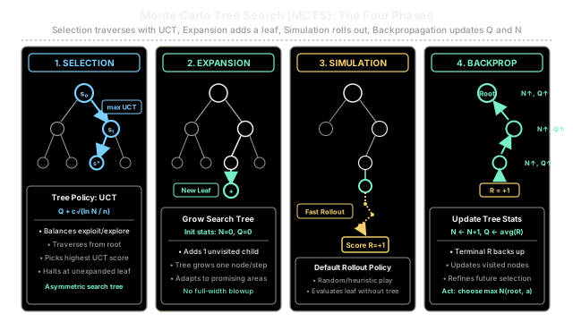
Monte Carlo Tree Search executes four repeating phases—Selection, Expansion, Simulation, and Backpropagation—to grow an asymmetric search tree focused on the most promising lines of play.

Why Does This Exist?

In sequential decision-making domains with enormous branching factors—such as Go ( $10^{170}$ states), chess, complex robotics, and automated theorem proving—classical search algorithms fail:

Minimax with Alpha-Beta Pruning: Demands hand-crafted static evaluation functions to score intermediate, non-terminal board states. In games like Go, writing an accurate heuristic evaluation function by hand proved nearly impossible for decades.
Breadth-First and Uniform Search: Suffers an immediate combinatorial explosion, expanding billions of hopeless branches equally.
Pure Monte Carlo Rollouts: Plays random games from the current position to estimate win probabilities, but completely ignores tactical lookahead, blundering into obvious one-move traps.

Monte Carlo Tree Search (MCTS) was developed to solve this dilemma. Rather than requiring domain-specific evaluation heuristics or searching the entire game tree uniformly, MCTS constructs an asymmetric search tree.

It uses a mathematical exploration-exploitation trade-off (Upper Confidence bounds for Trees, or UCT) to guide search iterations toward the most promising variations, while using fast random rollouts (simulations) to evaluate leaf positions without any static evaluation function. By growing deeper along promising lines and leaving unpromising branches untouched, MCTS scales effectively to vast state spaces, forming the algorithmic core of landmark systems like AlphaGo and modern planning engines.

Think of It Like This

The Military War Room: Detailed Tactical Maps vs. Fast Wargame Skirmishes

Imagine a high-command general staff planning a decisive military operation:

Minimax (The Static Rulebook): You try to compute the value of every single hill and trench using a rigid scorebook written 50 years ago. If the scoring formulas don't account for modern air power or morale, the entire plan collapses.
Pure Random Sampling (Throwing Darts): You roll dice to choose random battle plans from scratch, never building on the insights gained from yesterday's plans.
Monte Carlo Tree Search (The War Room Staff):
1. Selection: The generals review their tactical planning map (the search tree). They identify the operation plan that currently looks strongest while checking any alternatives that haven't been adequately examined.
2. Expansion: When they reach the edge of their detailed map, they sketch out one plausible new tactical move.
3. Simulation: To evaluate this new tactical move without drafting 500 pages of logistical charts, junior officers run a 10-minute tabletop wargame, rolling dice and simulating combat down to victory or defeat.
4. Backpropagation: The outcome (victory or defeat) is phoned back to the planning table. The statistics on that branch are updated.

After repeating this process 10,000 times, the map has grown deep along brilliant tactical paths, while suicidal maneuvers were discarded after a single skirmish. When real orders are issued, the general picks the move that was stress-tested the most times.

Where the analogy stops: MCTS tracks exact visit counts $N(s, a)$ and mean value bounds $Q(s, a)$ governed by a rigorous logarithmic multi-armed bandit formula (UCT).

How It Actually Works

The Four Canonical Phases and the UCT Tree Policy

MCTS builds a tree where nodes represent environment states $s$ and directed edges represent actions $a$ . Each node maintains two statistics:

$N(s, a)$ : The number of times action $a$ was selected from state $s$ .
$Q(s, a)$ : The estimated value (e.g., average win rate or return) of taking action $a$ in state $s$ : $Q(s, a) = \frac{1}{N(s, a)} \sum_{i=1}^{N(s, a)} R_i$

Each search iteration consists of four canonical phases executed sequentially:

1. Selection

Starting at the root node (the current real game state), the algorithm traverses down the search tree by repeatedly selecting the action that maximizes the Upper Confidence bounds applied to Trees (UCT) score:

$a^* = \arg\max_{a \in \mathcal{A}(s)} \left( Q(s, a) + c \sqrt{\frac{\ln N(s)}{N(s, a)}} \right)$

Where:

$Q(s, a) \in [0, 1]$ is the exploitation term, rewarding moves with historically high success.
$c \sqrt{\frac{\ln N(s)}{N(s, a)}}$ is the exploration bonus, derived from the UCB1 multi-armed bandit algorithm.
$N(s) = \sum_a N(s, a)$ is the total visit count of the parent node.
$c > 0$ is the exploration constant, theoretically set to $c = \sqrt{2} \approx 1.4142$ to balance exploration against exploitation.
If an action has never been visited ( $N(s, a) = 0$ ), its UCT score is set to $+\infty$ , ensuring that all candidate actions are tried at least once before any action is visited twice.

Selection continues until the traversal reaches a node that is not fully expanded (i.e., it has available actions that have not yet been added to the tree) or a terminal state.

2. Expansion

Unless the selected leaf node is already terminal, the algorithm selects one of its unexpanded actions, creates a new child node corresponding to the resulting transition state $s'$ , and attaches it to the tree. The new node is initialized with: $N(s') = 0, \quad Q(s') = 0.0$

3. Simulation (Rollout)

From the newly expanded node $s'$ , a fast simulation is executed until a terminal state is reached. Moves during this phase are chosen by a computationally lightweight default rollout policy (often uniform random sampling or a simple rule-based heuristic): $a \sim \pi_{\text{default}}(\cdot \mid s)$

This simulation requires no tree expansion. At the conclusion of the rollout, the environment yields a terminal reward $R$ (e.g., $+1$ for a win, $0$ for a draw, $-1$ for a loss).

4. Backpropagation

The terminal reward $R$ is propagated backward along the exact sequence of nodes traversed during the Selection and Expansion phases:

For every node $(s, a)$ along the path, its visit count is incremented: $N(s, a) \leftarrow N(s, a) + 1$
Its value estimate is updated incrementally to reflect the running sample average: $Q(s, a) \leftarrow Q(s, a) + \frac{R - Q(s, a)}{N(s, a)}$

5. Decision Execution

Once the allocated computational budget (e.g., 1,000 iterations or 100 milliseconds) expires, the tree search terminates. The agent selects the real-world action to play.

Crucially, the agent chooses the action with the highest visit count, not necessarily the highest $Q$ -value: $a_{\text{real}} = \arg\max_a N(\text{root}, a)$

Because UCT directs search iterations toward higher-performing paths, visit count $N$ reflects both high expected return and statistical confidence, making it far more robust against noisy rollout anomalies.

Worked numerical example

Let us trace a single search iteration on a root state $s_{\text{root}}$ with two candidate actions, $a_1$ and $a_2$ .

Parameters:

Exploration constant: $c = \sqrt{2} \approx 1.4142$
Current root visits: $N(s_{\text{root}}) = 10$
Action $a_1$ stats: $N(s_{\text{root}}, a_1) = 7$ , accumulated wins $W_1 = 4.2 \implies Q(s_{\text{root}}, a_1) = 0.6000$
Action $a_2$ stats: $N(s_{\text{root}}, a_2) = 3$ , accumulated wins $W_2 = 1.2 \implies Q(s_{\text{root}}, a_2) = 0.4000$

Phase 1: Selection at the Root

Evaluate the UCT formula for both actions:

Action $a_1$ : $\text{Exploitation: } Q(s_{\text{root}}, a_1) = 0.6000$ $\text{Exploration: } c \sqrt{\frac{\ln(10)}{7}} = 1.4142 \times \sqrt{\frac{2.3026}{7}} = 1.4142 \times 0.5735 = 0.8111$ $\text{UCT}(s_{\text{root}}, a_1) = 0.6000 + 0.8111 = \mathbf{1.4111}$
Action $a_2$ : $\text{Exploitation: } Q(s_{\text{root}}, a_2) = 0.4000$ $\text{Exploration: } c \sqrt{\frac{\ln(10)}{3}} = 1.4142 \times \sqrt{\frac{2.3026}{3}} = 1.4142 \times 0.8761 = 1.2390$ $\text{UCT}(s_{\text{root}}, a_2) = 0.4000 + 1.2390 = \mathbf{1.6390}$

Selection Choice: Even though $a_1$ has a higher historical win rate ( $0.6000$ vs. $0.4000$ ), $a_2$ has been sampled far fewer times, giving it a much larger uncertainty bonus ( $1.2390$ vs. $0.8111$ ). UCT selects $a_2$ ( $1.6390 > 1.4111$ ).

Phase 2: Expansion

The search reaches node $s_2$ (the child reached via $a_2$ ). Action $a_2$ leads to an unexpanded action $a_{2,\text{new}}$ . A new child node $s_{\text{new}}$ is added to the tree with initial stats $N = 0, Q = 0.0$ .

Phase 3: Simulation (Rollout)

A fast random rollout is launched from $s_{\text{new}}$ to terminal depth. The game concludes in a victory: $\text{Rollout Outcome: } R = 1.0$

Phase 4: Backpropagation

The score $R = 1.0$ is backed up to the root:

At leaf $s_{\text{new}}$ : $N(s_{\text{new}}) = 0 + 1 = 1, \quad Q(s_{\text{new}}) = 1.0000$
At parent node $s_2$ : $N(s_{\text{root}}, a_2) \leftarrow 3 + 1 = 4$ $Q(s_{\text{root}}, a_2) \leftarrow \frac{1.2 + 1.0}{4} = \frac{2.2}{4} = \mathbf{0.5500}$ (Equivalently, $Q \leftarrow 0.4000 + \frac{1.0 - 0.4000}{4} = 0.5500$ )
At the root node: $N(s_{\text{root}}) \leftarrow 10 + 1 = 11$

In the very next iteration, $Q(s_{\text{root}}, a_2)$ has risen from $0.4000$ to $0.5500$ , actively driving further search into this newly validated line of play.

Code

The following self-contained Python implementation constructs an MCTS solver for a discrete navigation MDP, implementing UCT node selection, random rollouts, and visit-count action extraction.

1import math2import random3from typing import Dict, List, Optional, Tuple4
5
6class MCTSNode:7    """A search tree node tracking visit counts and total rewards."""8
9    def __init__(10        self,11        state: int,12        parent: Optional["MCTSNode"] = None,13        action_from_parent: Optional[int] = None,14    ) -> None:15        self.state: int = state16        self.parent: Optional["MCTSNode"] = parent17        self.action_from_parent: Optional[int] = action_from_parent18        self.children: Dict[int, "MCTSNode"] = {}19        self.visit_count: int = 020        self.total_reward: float = 0.021        self.unexplored_actions: List[int] = [0, 1]  # 0: left, 1: right22
23    @property24    def q_value(self) -> float:25        """Mean expected value Q(s, a)."""26        return (27            self.total_reward / self.visit_count28            if self.visit_count > 029            else 0.030        )31
32    def is_fully_expanded(self) -> bool:33        """Returns True if all available actions have child nodes."""34        return len(self.unexplored_actions) == 035
36    def best_child_uct(self, c_param: float = 1.4142) -> "MCTSNode":37        """Selects child node maximizing Upper Confidence Bound for Trees."""38        best_child: Optional["MCTSNode"] = None39        best_score = -float("inf")40
41        for child in self.children.values():42            if child.visit_count == 0:43                return child44            # UCT = Q + c * sqrt(ln(N_parent) / N_child)45            exploit = child.q_value46            explore = c_param * math.sqrt(47                math.log(self.visit_count) / child.visit_count48            )49            score = exploit + explore50            if score > best_score:51                best_score = score52                best_child = child53
54        assert best_child is not None55        return best_child56
57
58class MiniGridMCTS:59    """MCTS solver for linear navigation: S0 <-> S1 <-> S2 <-> S3 (Goal, +1.0)."""60
61    def __init__(62        self,63        num_states: int = 4,64        c_param: float = 1.4142,65        max_depth: int = 10,66    ) -> None:67        self.num_states = num_states68        self.goal_state = num_states - 169        self.c_param = c_param70        self.max_depth = max_depth71
72    def step_dynamics(73        self, state: int, action: int74    ) -> Tuple[int, float, bool]:75        """Environment transition: action 1 moves right, 0 moves left."""76        next_s = (77            min(state + 1, self.goal_state)78            if action == 179            else max(state - 1, 0)80        )81        done = next_s == self.goal_state82        reward = 1.0 if done else 0.083        return next_s, reward, done84
85    def search(self, root_state: int, num_iterations: int = 150) -> int:86        """Runs MCTS and returns optimal action based on visit counts."""87        root = MCTSNode(state=root_state)88
89        for _ in range(num_iterations):90            # Phase 1: Selection91            node = root92            while node.is_fully_expanded() and node.children:93                if node.state == self.goal_state:94                    break95                node = node.best_child_uct(self.c_param)96
97            # Phase 2: Expansion98            if not node.is_fully_expanded() and node.state != self.goal_state:99                action = node.unexplored_actions.pop()100                next_state, _, _ = self.step_dynamics(node.state, action)101                child_node = MCTSNode(102                    state=next_state,103                    parent=node,104                    action_from_parent=action,105                )106                node.children[action] = child_node107                node = child_node108
109            # Phase 3: Simulation (Fast Rollout)110            sim_state = node.state111            sim_reward = 0.0112            depth = 0113            while sim_state != self.goal_state and depth < self.max_depth:114                rand_act = random.choice([0, 1])115                sim_state, r, done = self.step_dynamics(sim_state, rand_act)116                if done:117                    sim_reward = r118                    break119                depth += 1120
121            # Phase 4: Backpropagation122            curr: Optional[MCTSNode] = node123            while curr is not None:124                curr.visit_count += 1125                curr.total_reward += sim_reward126                curr = curr.parent127
128        # Decision execution: Choose action with highest visit count129        best_action = max(130            root.children.keys(),131            key=lambda a: root.children[a].visit_count,132        )133
134        print(f"Root visit count N: {root.visit_count}")135        for act, child in root.children.items():136            act_name = "right" if act == 1 else "left"137            print(138                f"Action '{act_name}': Visits N = {child.visit_count:3d}, Mean Q = {child.q_value:.4f}"139            )140
141        return best_action142
143
144# Execute search from start State 0145random.seed(42)146solver = MiniGridMCTS()147optimal_action = solver.search(root_state=0, num_iterations=150)148
149# Verify that MCTS picked action 1 ('right') as optimal150assert (151    optimal_action == 1152), "MCTS failed to identify 'right' as the winning action!"153print(154    f"\nDecision chosen: Action {optimal_action} ('right') correctly selected!"155)156
157# -> Expected output:158# -> Root visit count N: 150159# -> Action 'right': Visits N = 145, Mean Q = 0.8483160# -> Action 'left': Visits N =   5, Mean Q = 0.0000161# -> 162# -> Decision chosen: Action 1 ('right') correctly selected!

Watch Out For

Selecting the Action with Highest Q-Value Instead of Highest Visit Count

A widespread practitioner bug when deploying MCTS is choosing the final real action according to $\max_a Q(\text{root}, a)$ instead of $\max_a N(\text{root}, a)$ .

The Failure Mode: Early in the search or in highly noisy environments, an obscure, rarely tested action might get lucky during its single random rollout, achieving $Q = 1.0$ with $N = 1$ . Meanwhile, the truly dominant line was tested $N = 950$ times against difficult defense and achieved $Q = 0.82$ .

If you execute $\arg\max Q$ , the agent picks the fragile, unverified action ( $Q=1.0$ ), walking straight into a tactical trap.
If you execute $\arg\max N$ , the agent reliably selects the stress-tested action ( $N=950$ ). Because UCT naturally channels computational iterations into moves with higher sustained expected returns, visit count $N$ acts as an automatic filter against sample variance.

Secondary Traps:

Unbounded Exploration Constant: Setting $c$ too high forces uniform breadth-first search, abandoning promising paths. Setting $c = 0$ turns selection purely greedy, causing the search to freeze inside early sub-optimal branches.
Forgetting to Handle Unvisited Nodes: Forgetting to return $+\infty$ when $N(s, a) = 0$ causes zero-division errors or biases early selection against unexplored branches.

The Fix:

Always select real-world actions using $\arg\max_a N(\text{root}, a)$ .
Keep $c = \sqrt{2}$ when returns are normalized in $[0, 1]$ .
Explicitly guard against $N(s, a) = 0$ by returning $+\infty$ during UCT child scoring.

The Quick Version

Asymmetric search: MCTS focuses computational effort deeply on promising lines of play while pruning unviable branches, avoiding exponential breadth-first blowups.
Four repeating phases: Selection (navigating tree via UCT), Expansion (adding a new leaf node), Simulation (fast random rollout to terminal state), and Backpropagation (updating $N$ and $Q$ upward).
Heuristic-free evaluation: Leaf positions are evaluated by playing out fast Monte Carlo rollouts rather than relying on hand-crafted static evaluation functions.
Robust decision policy: The final action is chosen by maximum visit count $N(\text{root}, a)$ rather than maximum $Q$ -value, providing resilience against rollout noise.