n-Step TD Prediction
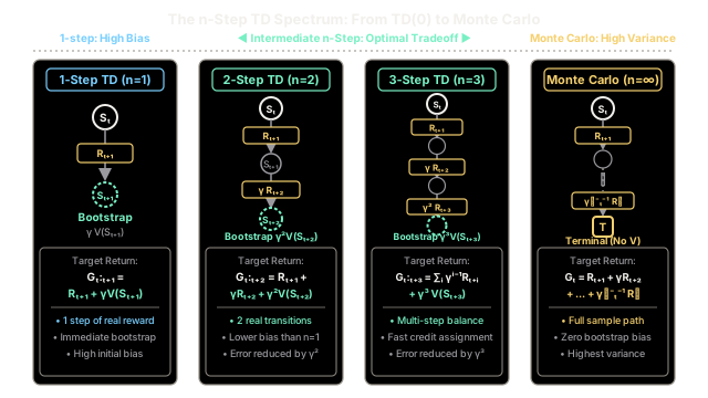
n-step TD prediction delays bootstrapping by looking ahead n transitions, letting you smoothly tune between the rapid low-variance updates of one-step TD and the unbiased trajectory sampling of Monte Carlo.
Why Does This Exist?
In reinforcement learning, estimating a state value function requires an update target. Classical methods stand at two opposing extremes of a fundamental trade-off:
- One-step Temporal Difference learning, or TD(0): Bootstraps immediately after experiencing a single transition (). The target is . Because it only depends on a single sample step, its variance is low. However, its target heavily relies on the current value estimate . If the initial value estimates are poorly calibrated, TD(0) injects substantial estimation bias into every update. Furthermore, a terminal reward must trickle backwards one transition per episode, requiring many episodes for distant states to learn.
- Monte Carlo (MC) prediction: Waits until the entire trajectory terminates () before computing the actual sample return . Because it uses actual realized rewards with zero bootstrapping, its target is completely unbiased. But accumulating dozens or hundreds of stochastic transitions introduces high sample variance. MC also cannot learn in non-terminating continuing tasks or mid-episode.
n-step TD prediction exists to bridge this gap. Instead of forcing an all-or-nothing choice between one step and complete termination, it parameterizes the lookahead horizon to an arbitrary integer . By accumulating steps of real environment transitions before substituting the remaining future with a bootstrapped value estimate, -step TD lets practitioners dial the exact sweet spot between bias and variance. Empirically, intermediate horizons (such as ) learn significantly faster and achieve lower asymptotic error than either extreme.
Think of It Like This
Performance Reviews: Daily Check-Ins vs. Quarterly Milestones vs. Retirement Retrospectives
Imagine evaluating the career trajectory and performance of a project lead:
- 1-Step TD (The Daily Check-In): At 5:00 PM on Monday, you observe today's output (). You then evaluate the lead's entire career value by combining Monday's output with your existing subjective hunch about where they will stand on Tuesday evening (). Because you only observed eight hours of real work, your review is dominated by your prior hunch. If your initial evaluation model is biased or flawed, your updates are distorted. Moreover, major breakthrough deliverables that take months to complete take forever to reflect in their Monday review.
- Monte Carlo (The Retirement Retrospective): You refuse to evaluate the project lead until they retire 35 years later (). You then calculate their true lifetime deliverables with zero guesswork. While this retrospective is completely free of subjective estimation bias, it comes decades too late to guide ongoing project decisions. Furthermore, 35 years of macroeconomic swings, team reorganizations, and random luck introduce enormous variance.
- n-Step TD (The Quarterly Milestone Review): You evaluate the lead after a defined 3-month project sprint ( months). You log 90 days of concrete, verifiable code commits, product releases, and customer feedback (). Only at that 3-month milestone do you combine those hard facts with an updated forecast for the remaining project roadmap (). You anchor the evaluation in substantial real data while keeping feedback timely enough to steer future work.
Where the analogy stops: In reinforcement learning, the future forecast is multiplied by an exact geometric discount factor , and updates are applied retroactively with an exact step size using a sliding trajectory buffer.
How It Actually Works
Multi-Step Bootstrapping and the Error Reduction Property
Consider an agent interacting with an environment in discrete time steps . At time step , the agent occupies state , takes action , transitions to state , and receives a scalar reward . The discount factor is , and the episode terminates at time step .
1. The n-Step Return
The core object of -step TD prediction is the -step return, denoted . It sums the first discounted rewards and bootstraps from the estimated value of the state visited steps into the future:
Where:
- is the reward observed at transition .
- discounts the reward received steps ahead.
- is the estimate of the value of state available at time .
- scales the bootstrapped value estimate.
If the trajectory reaches or surpasses terminal time step (that is, ), the return is simply truncated at , and no bootstrapping occurs because the value of a terminal state is identically zero:
Notice the two boundary conditions:
- When : , which is the standard one-step TD target.
- When (or ): , which is the complete Monte Carlo return.
2. The Value Update Rule
Because computing requires knowledge of transitions up to time step , the update for state cannot be executed at time . It is delayed until time .
Let denote the index of the state being updated. When the agent reaches time step (for ), it updates the value of the state visited at time :
Where:
- is the step-size learning rate.
- is the -step TD error.
- All other state estimates remain unchanged: for all .
When the episode terminates at step , the agent must drain its buffer by continuing to apply updates for all remaining historical states until every visited state has been updated.
3. Theoretical Guarantee: The Error Reduction Property
Why is multi-step bootstrapping guaranteed to behave well? Sutton and Barto established the error reduction property of -step returns:
Where is the true underlying value under policy .
This theorem proves that the expected -step return is guaranteed to be a strictly better estimate of than the current estimate , shrinking the worst-case error by a geometric factor of at least . As increases, the worst-case bias decays exponentially at rate .
Worked numerical example
To see how -step returns accelerate reward propagation, let us trace a single episode through a 5-step deterministic trajectory:
Let:
- Discount factor
- Step size
- Initial value estimates for all states: for all
We will compare the update applied to the starting state across , , , and Monte Carlo ():
Case 1: One-Step TD ()
At time step , the agent observes transition with reward .
The large downstream reward has zero impact on in this episode.
Case 2: Two-Step TD ()
At time step , the agent has observed with rewards .
Now directly benefits from both and , nearly tripling its value adjustment.
Case 3: Three-Step TD ()
At time step , the agent has observed transitions up to with rewards .
Case 4: Full Monte Carlo (, Horizon Reaches Terminal )
At time step , the terminal state is reached.
Comparison Across the Full Episode
When the episode finishes and all buffered updates are drained, the learned values across all states are:
| Method | ||||
|---|---|---|---|---|
| (TD(0)) | ||||
| (MC) |
Notice how the terminal reward propagates backwards:
- In , it only reaches .
- In , it reaches and .
- In , it reaches , and .
- In Monte Carlo, it travels all the way back to in a single episode.
Code
The following self-contained Python implementation processes an episodic trajectory using an explicit sliding window update buffer, properly handling the delayed updates and the end-of-episode draining phase.
from typing import Dict, List, Optional, Tuple
def n_step_td_prediction( trajectory: List[Tuple[str, float]], n: int, gamma: float = 0.9, alpha: float = 0.5, initial_values: Optional[Dict[str, float]] = None,) -> Dict[str, float]: """Computes state value estimates using episodic n-step TD prediction.
Args: trajectory: List of (state, reward) tuples where reward is received upon entering state. First element is (S0, 0.0); last is (Terminal, final_reward). n: Number of lookahead steps before bootstrapping (n >= 1). gamma: Discount factor in [0, 1]. alpha: Step size learning rate in (0, 1]. initial_values: Optional initial state values dictionary.
Returns: Dictionary mapping non-terminal state identifiers to updated values. """ states = [step[0] for step in trajectory] rewards = [step[1] for step in trajectory] total_steps = len(trajectory) - 1 # Terminal step T
# Initialize value dictionary v_table = ( {s: 0.0 for s in set(states)} if initial_values is None else initial_values.copy() ) terminal_state = states[total_steps] v_table[terminal_state] = 0.0 # Terminal state value is always 0.0
t = 0 while True: # tau is the index of the state whose estimate is currently being updated tau = t - n + 1
if tau >= 0: # 1. Sum observed rewards from step tau + 1 up to min(tau + n, T) g_return = 0.0 horizon = min(tau + n, total_steps) for i in range(tau + 1, horizon + 1): discount_power = i - tau - 1 g_return += (gamma**discount_power) * rewards[i]
# 2. Add bootstrapped value estimate only if horizon does not reach terminal step if tau + n < total_steps: bootstrapped_state = states[tau + n] g_return += (gamma**n) * v_table[bootstrapped_state]
# 3. Apply gradient-descent update rule to state S_tau state_to_update = states[tau] v_table[state_to_update] += alpha * ( g_return - v_table[state_to_update] )
# Termination condition: last updated state is T - 1 if tau == total_steps - 1: break
t += 1
return { s: round(v_table[s], 4) for s in sorted(v_table.keys()) if s != terminal_state }
# Trajectory: S0 -> (R=1.0) -> S1 -> (R=2.0) -> S2 -> (R=0.0) -> S3 -> (R=10.0) -> S4 (Terminal)example_trajectory = [ ("S0", 0.0), ("S1", 1.0), ("S2", 2.0), ("S3", 0.0), ("S4", 10.0),]
print("n=1 (TD(0)):", n_step_td_prediction(example_trajectory, n=1))print("n=2: ", n_step_td_prediction(example_trajectory, n=2))print("n=3: ", n_step_td_prediction(example_trajectory, n=3))print("n=4 (MC): ", n_step_td_prediction(example_trajectory, n=4))
# -> Expected output:# -> n=1 (TD(0)): {'S0': 0.5, 'S1': 1.0, 'S2': 0.0, 'S3': 5.0}# -> n=2: {'S0': 1.4, 'S1': 1.0, 'S2': 4.5, 'S3': 5.0}# -> n=3: {'S0': 1.4, 'S1': 5.05, 'S2': 4.5, 'S3': 5.0}# -> n=4 (MC): {'S0': 5.045, 'S1': 5.05, 'S2': 4.5, 'S3': 5.0}Watch Out For
Terminal Boundary Off-by-One and Phantom Bootstrapping
A prevalent bug when implementing -step TD is blindly adding the bootstrapped term without checking whether the lookahead index has surpassed the episode boundary .
The Failure Mode: When an agent approaches the end of an episode, frequently equals or exceeds . If the code does not clamp the reward summation at and unconditionally includes a bootstrap term, two severe errors occur:
- Out-of-Bounds Exceptions: Attempting to query
states[tau + n]crashes with an indexing exception. - Phantom Value Bleed: If the lookup wraps around or indexes a non-zero terminal value, the algorithm adds a "phantom" bootstrap value into the return. This injects artificial bias into terminal transitions, causing value estimates near episode goals to diverge.
- Premature Loop Termination: Ceasing execution as soon as without draining the buffer drops the final states () without ever updating them.
The Fix:
- Accumulate discounted rewards strictly up to .
- Add the bootstrapped value if and only if .
- Continue the outer loop until to ensure all remaining states in the sliding buffer receive their updates before the episode finishes.
The Quick Version
- Tunable spectrum: -step TD prediction bridges 1-step TD(0) and full Monte Carlo, letting you select an intermediate horizon that balances bootstrapping bias against trajectory variance.
- Delayed updates: Updates to state are computed at time , requiring a memory buffer of size to store recent states and rewards.
- Faster reward propagation: Increasing propagates terminal rewards multiple steps backwards within a single episode, eliminating the single-transition bottleneck of TD(0).
- Error reduction guarantee: The expected -step return is guaranteed to contract the maximum value error by at least , ensuring stable convergence toward the true value function .