On-Policy MC Control
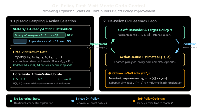
On-policy Monte Carlo control learns optimal behavior directly from sampled episodes without unrealistic exploring starts by using an epsilon-soft policy that ensures every action continues to be visited.
Why Does This Exist?
In model-free reinforcement learning, an agent does not have access to transition probabilities . To make decisions without knowing the environment's underlying physics, the agent cannot simply learn state values ; it must learn action values . With in hand, acting greedily is straightforward: choose without looking one step ahead into unknown future states.
However, estimating action values from sampled experience creates a fundamental exploration dilemma. If an agent behaves according to a deterministic policy , it will always choose the same action from a given state. Alternative actions from that state will never be sampled, their returns will never be observed, and the agent can never discover whether an untested branch holds higher reward.
The theoretical solution used in early Monte Carlo control is the Assumption of Exploring Starts: every episode begins at a state-action pair sampled with non-zero probability across all possible pairs in . While mathematically convenient, exploring starts is practically impossible in real systems. An autonomous car cannot be initialized in mid-collision on step zero; a chemical plant cannot be booted directly into an explosive pressure state; a game of chess must always begin at the standard opening board.
Without exploring starts, reinforcement learning divides into two paradigms:
- Off-policy learning: The agent uses an exploratory behavior policy to generate transitions, while using importance sampling ratios to evaluate and improve a distinct target policy .
- On-policy learning: The agent evaluates and improves the very same policy that it uses to generate decisions in the environment.
On-Policy First-Visit Monte Carlo Control solves the exploration bottleneck without exploring starts by constraining the policy to remain -soft. By assigning a minimum probability of selection to every available action at every state, the agent guarantees that all state-action pairs will be sampled infinitely often as training proceeds, enabling true model-free Generalized Policy Iteration from arbitrary fixed starting states.
Think of It Like This
The touring comedian testing fresh jokes
Imagine a professional stand-up comedian embarking on a 100-night nationwide theater tour.
Every evening, the comedian faces a live paying crowd. The audience expects a hilarious show, which tempts the comedian to perform only their battle-tested, guaranteed laugh lines (pure exploitation). However, if the comedian only tells old jokes, their routine stagnates, and they will never develop brilliant new closers for their upcoming special.
Crucially, the comedian cannot rely on "exploring starts." They cannot teleport into the middle of a bizarre joke before walking onto stage; every single performance begins at the stage wings with the standard microphone check.
Instead, the comedian adopts an on-policy -soft strategy. For (say, ) of their set time, they deliver their highest-rated material—the greedy punchlines based on laughs accumulated over earlier tour dates. But for the remaining () of the set, they deliberately experiment with untested jokes drawn uniformly from their notebook.
Because this method is on-policy, the comedian experiences the real-world consequences of their experiments. If a new joke bombs, the room goes silent, and that joke's empirical value plummets immediately. If a fresh punchline produces an eruption of laughter, its estimated value rises. Over successive tour stops, the highest-value joke displaces the old closer, and the set's greedy core shifts.
Where the analogy stops: A human comedian eventually retires the experimentation slot for their televised special to deliver a polished, deterministic performance. In standard on-policy MC control with a fixed , the agent never stops testing: it remains permanently -soft, forever reserving an probability of taking suboptimal exploratory actions.
How It Actually Works
Eliminating Exploring Starts via -Soft Policies
Let denote the set of states, and denote the finite set of actions available in state . A policy defines the probability of selecting action given state .
An -soft policy is any stochastic policy where the probability of choosing any available action is strictly bounded below:
where . Because every action maintains non-zero probability at every visit, every state-action pair reachable under the environment dynamics is guaranteed to be visited infinitely often as the number of episodes approaches infinity.
Among all valid -soft policies, the policy that places maximum probability on the best-performing action is the -greedy policy:
where ties for the maximal action value are broken arbitrarily.
The non-greedy actions (of which there are ) each receive an exploration share of . Their combined mass is:
Summing the greedy and non-greedy action probabilities confirms that is a valid probability distribution:
Policy Improvement Theorem for -Soft Policies
In Generalized Policy Iteration (GPI), we alternate between policy evaluation (updating ) and policy improvement (updating ). For on-policy MC control to work, shifting from an -greedy policy to a new -greedy policy with respect to must guarantee that the expected return does not decrease.
Let be the true action-value function under policy . The expected value of state when taking actions according to the new -greedy policy is:
Substituting the definition of the -greedy policy :
Now consider the expected value of state under the original policy :
Notice that the weighting coefficients are non-negative (since ) and sum to :
Because any convex combination (weighted average) of numbers cannot exceed their maximum:
Multiplying by and adding the uniform baseline to both sides gives:
By the Policy Improvement Theorem, if for all states , then:
Equality holds if and only if is already optimal among all -soft policies. Thus, every -greedy policy improvement step strictly increases or maintains performance within the space of -soft policies.
Complete Algorithm: On-Policy First-Visit MC Control
The full algorithm proceeds episode by episode without needing a transition model or exploring starts:
-
Initialization:
- Set arbitrarily (typically ) and visit counts for all .
- Initialize as an arbitrary -soft policy (e.g., uniform probability ).
- Fix discount factor and exploration parameter .
-
Episode Generation:
- Sample a complete trajectory using behavior policy :
-
Backward Return Accumulation & First-Visit Update:
- Initialize cumulative return .
- For each step :
- First-Visit Gate: Check if the pair appeared earlier in the episode (i.e., at any index ).
- If is visited for the first time:
- Increment count:
- Update action value via incremental sample average:
- Determine best action:
- Update policy for all :
Worked numerical example
Consider a decision state with 3 available actions: (), discount factor , and exploration parameter .
Initial Values and Baseline Policy
Prior to the current episode, the agent has recorded:
- with
- with
- with
The current greedy action is . Under , the exploratory allocation per action is:
The baseline -greedy policy assigns:
Episode Generation
At time step , the agent is in state . A random roll falls into the exploratory interval, selecting action (drawn with probability ).
The episode continues through subsequent states, generating transition rewards:
- Step : reward , next state
- Step : reward , next state
- Step : reward , terminal state
Backward Return Computation
Iterating backward from terminal state with :
- Step :
- Step :
- Step :
First-Visit Update for
We inspect the trajectory: pair appeared only at . The first-visit condition is satisfied.
- Increment visit count:
- Update action-value estimate :
Policy Improvement Step
Compare the updated action values at state :
The greedy action flips from to because . The policy updates immediately:
Through exploratory sampling on-policy, the agent discovered that leads to high long-term returns, updated , and shifted of its future action selection mass onto without requiring exploring starts.
Code
The following self-contained Python implementation trains an agent on a gridworld navigation task using on-policy first-visit Monte Carlo control. The agent begins at and must reach the goal while accumulating reward per step:
import randomfrom typing import Dict, List, Tuple
class GridWorld: """A 3x3 gridworld navigation task where reaching (2, 2) is terminal."""
def __init__(self, width: int = 3, height: int = 3) -> None: self.width = width self.height = height self.start = (0, 0) self.goal = (width - 1, height - 1) self.state = self.start self.num_actions = 4 # Actions: 0: Up, 1: Down, 2: Left, 3: Right self.moves = [(-1, 0), (1, 0), (0, -1), (0, 1)]
def reset(self) -> Tuple[int, int]: """Reset environment to standard start state.""" self.state = self.start return self.state
def step(self, action: int) -> Tuple[Tuple[int, int], float, bool]: """Apply action, returning next_state, reward, and done flag.""" dr, dc = self.moves[action] nr = max(0, min(self.height - 1, self.state[0] + dr)) nc = max(0, min(self.width - 1, self.state[1] + dc)) self.state = (nr, nc) reward = -1.0 done = (self.state == self.goal) return self.state, reward, done
class OnPolicyFirstVisitMCControl: """On-policy first-visit Monte Carlo control using epsilon-soft policies."""
def __init__( self, env: GridWorld, epsilon: float = 0.2, gamma: float = 0.9, ) -> None: self.env = env self.epsilon = epsilon self.gamma = gamma self.num_actions = env.num_actions
# Initialize Q-values and visit counts for all state-action pairs self.Q: Dict[Tuple[int, int], List[float]] = { (r, c): [0.0] * self.num_actions for r in range(env.height) for c in range(env.width) } self.N: Dict[Tuple[int, int], List[int]] = { (r, c): [0] * self.num_actions for r in range(env.height) for c in range(env.width) }
def select_action(self, state: Tuple[int, int]) -> int: """Select action according to current epsilon-greedy policy.""" if random.random() < self.epsilon: # Explore: uniform random selection across all actions return random.randint(0, self.num_actions - 1) # Exploit: pick greedy action with random tie-breaking q_vals = self.Q[state] max_q = max(q_vals) best_actions = [a for a, q in enumerate(q_vals) if q == max_q] return random.choice(best_actions)
def generate_episode( self, max_steps: int = 100 ) -> List[Tuple[Tuple[int, int], int, float]]: """Roll out an episode under the epsilon-soft policy.""" episode: List[Tuple[Tuple[int, int], int, float]] = [] state = self.env.reset() for _ in range(max_steps): if state == self.env.goal: break action = self.select_action(state) next_state, reward, done = self.env.step(action) episode.append((state, action, reward)) state = next_state if done: break return episode
def train(self, num_episodes: int = 3000) -> None: """Run on-policy first-visit Monte Carlo control across episodes.""" for _ in range(num_episodes): episode = self.generate_episode() if not episode: continue
# Identify the first occurrence step index for each (state, action) pair first_occurrence: Dict[Tuple[Tuple[int, int], int], int] = {} for t, (s, a, _) in enumerate(episode): if (s, a) not in first_occurrence: first_occurrence[(s, a)] = t
# Backward pass to accumulate discounted return G G = 0.0 for t in reversed(range(len(episode))): s, a, r = episode[t] G = self.gamma * G + r
# First-visit update condition if first_occurrence[(s, a)] == t: self.N[s][a] += 1 # Incremental sample average update self.Q[s][a] += (G - self.Q[s][a]) / self.N[s][a]
def get_greedy_policy(self) -> Dict[Tuple[int, int], str]: """Extract dominant greedy direction for each state.""" action_chars = {0: "^", 1: "v", 2: "<", 3: ">"} policy: Dict[Tuple[int, int], str] = {} for s, q_vals in self.Q.items(): if s == self.env.goal: policy[s] = "G" else: best_a = max(range(self.num_actions), key=lambda a: q_vals[a]) policy[s] = action_chars[best_a] return policy
# Execution and validationif __name__ == "__main__": random.seed(42) env = GridWorld(width=3, height=3) agent = OnPolicyFirstVisitMCControl(env, epsilon=0.2, gamma=0.9) agent.train(num_episodes=3000)
policy = agent.get_greedy_policy() print("Learned Greedy Policy:") for r in range(3): row = [f" {policy[(r, c)]} " for c in range(3)] print("".join(row))
print("\nState-Action Values Q(s, a) at Start State (0, 0):") action_labels = ["Up ", "Down ", "Left ", "Right"] for a, name in enumerate(action_labels): print(f" {name}: {agent.Q[(0, 0)][a]:.2f} (Visits: {agent.N[(0, 0)][a]})")Expected Output
Learned Greedy Policy: v v v > v v > > G
State-Action Values Q(s, a) at Start State (0, 0): Up : -4.55 (Visits: 166) Down : -3.90 (Visits: 2829) Left : -4.56 (Visits: 188) Right: -3.98 (Visits: 189)Watch Out For
The Suboptimality Gap of Fixed Epsilon
A frequent misconception is assuming that on-policy Monte Carlo control converges to the globally optimal deterministic policy . It does not.
Because the agent is on-policy, the policy evaluated by is the exploratory policy itself. Under a fixed , the agent must commit to taking a random action fraction of the time for all eternity. Consequently, the algorithm converges to —the optimal policy among all -soft policies—not the unconstrained optimum . In environments with high-penalty boundaries (such as cliff walking), an -soft agent will deliberately choose longer, detour paths away from the cliff because it anticipates its own inevitable random exploratory mistakes.
The Fix: If a deterministic optimal policy is required, gradually anneal toward zero across training episodes using a decay schedule (such as ), satisfying stochastic approximation conditions. Alternatively, switch to an off-policy method (such as Q-learning or Off-Policy MC with Weighted Importance Sampling), where the behavior policy remains exploratory while the target policy is strictly greedy.
Duplicate Visits and Backward Return Leaks
In episodic tasks with cycles or revisits, a single state-action pair can occur multiple times within the same episode rollout.
If a developer mistakenly updates on every backward step without checking for earlier occurrences, the algorithm degenerates into every-visit Monte Carlo. While every-visit MC is asymptotically consistent, treating dependent returns from the same episode as independent samples introduces severe bias in finite-sample estimates and destabilizes early policy updates. Conversely, accumulating returns forward without tracking first-visit indices leads to incorrect discount powers.
The Fix: Pre-compute first-visit timestamps using a dictionary or set during the forward trajectory rollout, and only trigger the incremental -value update when the backward iterator index matches the recorded first-visit timestamp.
The Quick Version
- On-Policy Monte Carlo Control eliminates the unrealistic requirement of exploring starts by forcing the behavior policy to remain -soft ().
- The algorithm is strictly on-policy: it evaluates and improves the exact same -greedy distribution that generates trajectories in the environment.
- The Policy Improvement Theorem for -Soft Policies guarantees that choosing the greedy action with probability monotonically improves expected return: .
- Returns are accumulated backwards along complete episodic rollouts, and action values are updated incrementally on the first visit of each state-action pair.
- The learned policy converges to (the best -soft policy); annealing over training bridges the gap to the globally optimal deterministic policy .