Monte Carlo Exploring Starts
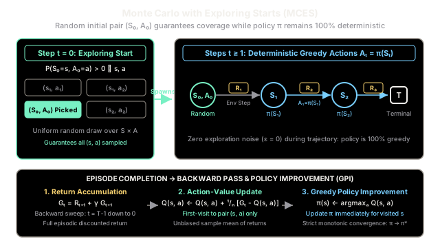
Monte Carlo with Exploring Starts guarantees comprehensive state-action exploration by beginning episodes at every state-action pair with non-zero probability.
Why Does This Exist?
In model-free reinforcement learning, finding an optimal policy requires learning action values . However, if an agent acts deterministically according to its current greedy policy, it will only ever experience the actions it already believes are best. Suboptimal early estimates can permanently lock the agent into choosing poor actions, leaving genuinely optimal paths unvisited.
Without an environment transition model, you cannot compute expectations across untried branches. The classic solution is the Exploring Starts assumption: guaranteeing that every possible state-action pair has a strictly positive probability of being chosen as the initial step of an episode. This ensures infinite exploration across all choices in the limit, allowing the agent to follow a purely greedy deterministic policy for all subsequent steps.
Think of It Like This
The Flight Simulator Scenario Selector
Imagine a flight simulator designed to train pilots for every emergency scenario. If the simulation always started on the runway on a calm sunny day, a pilot following standard procedure would never experience engine failure at 30,000 feet or crosswind landings at night.
To ensure complete competence across the entire state-action space, the flight instructor uses an exploring starts protocol: the simulator initializes the airplane at an arbitrarily chosen altitude, airspeed, and weather condition, with the pilot forced to take a specific initial control input (e.g., full left rudder). Once that first step is taken, the pilot is evaluated purely on their standard emergency playbook. Over thousands of simulated flights starting from every possible altitude and rudder position, every action in every state is thoroughly evaluated without having to introduce random control wobbles during normal flight.
How It Actually Works
The Exploring Starts Protocol and Policy Iteration
Monte Carlo with Exploring Starts (MCES) alternates between sample-based policy evaluation and greedy policy improvement:
- Episode Initialization: Select and such that for all .
- Deterministic Trajectory: For , sample actions strictly according to the current deterministic policy:
- Return Computation: Backward iterate from terminal time to compute returns:
- Value Update (First-Visit): For each pair appearing in the episode, record the first occurrence time :
- Greedy Improvement: Update the policy immediately for each state visited:
Because exploring starts handles the exploration burden on step , the policy does not need an exploration parameter like . It remains purely deterministic and greedy.
Worked numerical example
Consider a simplified grid navigation task with states and actions . The discount factor is .
Suppose initial estimates are , , meaning the initial greedy policy is .
- Episode 1: Exploring starts selects and forces exploratory action .
- The transition yields reward and transitions to .
- From , the agent follows , receives , and reaches the terminal state.
- Return Calculation:
- Value Update:
- Prior , prior .
- New count .
- Updated .
- Policy Improvement:
- Compare .
- The greedy policy updates: .
The forced initial exploration discovered a path worth that the initial greedy policy would have ignored forever.
Code
from collections import defaultdictimport random
class MonteCarloExploringStarts: def __init__(self, states: list[str], actions: list[str], gamma: float = 0.9): self.states = states self.actions = actions self.gamma = gamma self.Q = defaultdict(float) self.returns_count = defaultdict(int) self.policy = {s: random.choice(actions) for s in states}
def generate_episode(self, env_step_fn) -> list[tuple[str, str, float]]: # Exploring starts: pick S0 and A0 uniformly at random s0 = random.choice(self.states) a0 = random.choice(self.actions) trajectory = []
s = s0 a = a0 while True: next_s, reward, done = env_step_fn(s, a) trajectory.append((s, a, reward)) if done: break s = next_s a = self.policy[s] # Strictly follow deterministic policy thereafter return trajectory
def update_policy(self, trajectory: list[tuple[str, str, float]]) -> None: G = 0.0 visited = set() # Backward return accumulation for s, a, r in reversed(trajectory): G = self.gamma * G + r
# First-visit MC update for the starting pair s0, a0, _ = trajectory[0] self.returns_count[(s0, a0)] += 1 n = self.returns_count[(s0, a0)] self.Q[(s0, a0)] += (G - self.Q[(s0, a0)]) / n
# Greedy policy improvement best_action = max(self.actions, key=lambda act: self.Q[(s0, act)]) self.policy[s0] = best_action
# Simulated 2-state environment stepdef dummy_env(s: str, a: str) -> tuple[str, float, bool]: if s == "S1" and a == "Right": return "S2", 4.0, False return "Terminal", 10.0, True
agent = MonteCarloExploringStarts(states=["S1", "S2"], actions=["Left", "Right"])sample_traj = [("S1", "Right", 4.0), ("S2", "Right", 10.0)]agent.update_policy(sample_traj)print("Updated Q(S1, Right):", agent.Q[("S1", "Right")])print("Updated Policy for S1:", agent.policy["S1"])# -> Updated Q(S1, Right): 13.0# -> Updated Policy for S1: RightWatch Out For
Physical Realizability in Real-World Systems
The Exploring Starts assumption is mathematically elegant in simulated environments like games or board scenarios, but it is physically impossible in most real-world applications. A real autonomous vehicle cannot be randomly initialized at perpendicular to oncoming highway traffic, and an industrial chemical reactor cannot be safely initialized at explosive core temperatures.
When exploring starts cannot be physically guaranteed, relying on this algorithm leads to complete policy stagnation. In these scenarios, use -soft on-policy control or off-policy importance sampling to explore safely from natural start states.
The Quick Version
- Exploring Starts guarantees that every state-action pair has non-zero probability of being the initial step of an episode.
- By guaranteeing exploration on step , the policy can remain strictly deterministic and greedy on all subsequent steps.
- Monte Carlo updates wait for episode termination and compute unbiased returns by backward accumulation.
- The assumption is viable in simulators and games but physically impractical in real-world robotics and industrial control.