Monte Carlo Control

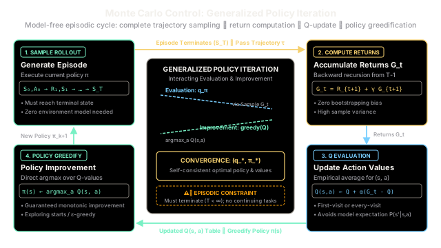
Why Does This Exist?

In classical planning frameworks like Dynamic Programming, finding an optimal policy requires full access to the environment's transition dynamics $P(s' \mid s, a)$ and reward distributions $R(s, a)$. However, in practical reinforcement learning problems—such as robotic manipulation, video games, or financial order routing—these governing probabilities are unknown or too intricate to compute analytically.

When dynamics are unknown, evaluating only state values $V(s)$ is not enough to make decisions. Under state values alone, selecting the greedy action requires computing:

$\pi'(s) = \arg\max_{a \in \mathcal{A}} \sum_{s' \in \mathcal{S}} P(s' \mid s, a) \left[ R(s, a, s') + \gamma V(s') \right]$

This one-step lookahead still depends explicitly on the transition distribution $P(s' \mid s, a)$. Without a transition model, the agent cannot evaluate which action leads to which successor states.

Monte Carlo control resolves this by shifting evaluation from state values $V(s)$ to state-action values $Q(s, a)$. By estimating the expected return of taking action $a$ in state $s$ directly from sample episodes, the agent can greedify its policy without any model:

$\pi'(s) = \arg\max_{a \in \mathcal{A}} Q(s, a)$

Unlike Temporal Difference Learning, which bootstraps value estimates from immediate subsequent states ($S_{t+1}$), Monte Carlo control samples complete episodes to calculate true discounted returns $G_t$. This eliminates bootstrapping bias completely and prevents divergence under function approximation in on-policy settings, providing a grounded framework for model-free policy optimization.

Think of It Like This

How It Actually Works

Generalized Policy Iteration with Monte Carlo Evaluation

Monte Carlo control applies the framework of Generalized Policy Iteration (GPI) to model-free settings. It alternates between two competing processes:

1. Policy Evaluation: Estimating action values $Q(s, a)$ from empirical trajectory rollouts generated under the current policy $\pi$.
2. Policy Improvement: Updating the policy greedily with respect to the updated action values $Q(s, a)$.

$\pi_0 \xrightarrow{\text{Evaluation}} Q^{\pi_0} \xrightarrow{\text{Improvement}} \pi_1 \xrightarrow{\text{Evaluation}} Q^{\pi_1} \xrightarrow{\text{Improvement}} \dots \to \pi^*, Q^*$

Mathematical Formulation

Consider a finite Markov Decision Process defined by the tuple $(\mathcal{S}, \mathcal{A}, P, R, \gamma)$. The agent executes policy $\pi$ to generate a complete episode terminating at time step $T$:

$\tau = (S_0, A_0, R_1, S_1, A_1, R_2, \dots, S_{T-1}, A_{T-1}, R_T, S_T)$

For each time step $t \in [0, T-1]$, the total discounted return $G_t$ is defined as:

$G_t \doteq \sum_{k=0}^{T - t - 1} \gamma^k R_{t+k+1} = R_{t+1} + \gamma G_{t+1}$

To estimate $Q^\pi(s, a) = \mathbb{E}_\pi [G_t \mid S_t = s, A_t = a]$, Monte Carlo evaluation tracks empirical returns:

• First-Visit MC: Updates $Q(s, a)$ using only the first occurrence of state-action pair $(s, a)$ within episode $\tau$.
• Every-Visit MC: Updates $Q(s, a)$ for every occurrence of $(s, a)$ within episode $\tau$.

Using an incremental sample average with visit count $N(s, a)$:

$N(S_t, A_t) \leftarrow N(S_t, A_t) + 1$

$Q(S_t, A_t) \leftarrow Q(S_t, A_t) + \frac{1}{N(S_t, A_t)} \left[ G_t - Q(S_t, A_t) \right]$

For non-stationary policies or tracking tracking shifting values across iterations, practitioners often use a constant step size $\alpha \in (0, 1]$:

$Q(S_t, A_t) \leftarrow Q(S_t, A_t) + \alpha \left[ G_t - Q(S_t, A_t) \right]$

Policy Greedification and Monotonic Improvement

Once action values are updated, policy improvement makes the policy greedy with respect to $Q$:

$\pi'(s) \leftarrow \arg\max_{a \in \mathcal{A}} Q(s, a)$

By the Policy Improvement Theorem, choosing the greedy action guarantees that the new policy $\pi'$ achieves expected returns greater than or equal to the previous policy $\pi$:

$q_\pi(s, \pi'(s)) = \max_{a \in \mathcal{A}} q_\pi(s, a) \ge q_\pi(s, \pi(s)) = v_\pi(s) \quad \forall s \in \mathcal{S}$

Because the state space is finite, repeated alternation between evaluation and improvement drives the policy toward the unique optimal policy $\pi^*$.

The Exploration Requirement

If policy $\pi$ becomes strictly deterministic, unchosen actions in state $s$ are never executed. Consequently, their action values $Q(s, a)$ receive no empirical returns and remain unrefined, risking premature convergence to suboptimal policies.

To ensure convergence, every state-action pair must be sampled infinitely often:

• Monte Carlo with Exploring Starts: Assumes every episode starts with a randomly selected state-action pair $(S_0, A_0)$, guaranteeing that all pairs are visited.
• $\epsilon$-Greedy Policies: Selects the greedy action with probability $1 - \epsilon + \frac{\epsilon}{|\mathcal{A}|}$, and explores random actions with probability $\frac{\epsilon}{|\mathcal{A}|}$, maintaining continual exploration throughout learning.

Worked numerical example

Consider an agent in decision state $s_0$ with discount factor $\gamma = 0.9$.

• Available actions at $s_0$: $a_{\text{safe}}$ and $a_{\text{risky}}$.
• Taking $a_{\text{safe}}$ transitions to intermediate state $s_1$ with immediate reward $R_1 = +1.0$. From $s_1$, the agent takes $a_{\text{proceed}}$ to reach terminal state $s_T$ with reward $R_2 = +4.0$.
• Taking $a_{\text{risky}}$ transitions directly to terminal state $s_T$ with reward $R_1 = +8.0$.

Initialize all tabular values to zero:

• $Q(s_0, a_{\text{safe}}) = 0.0$, $N(s_0, a_{\text{safe}}) = 0$
• $Q(s_0, a_{\text{risky}}) = 0.0$, $N(s_0, a_{\text{risky}}) = 0$
• $Q(s_1, a_{\text{proceed}}) = 0.0$, $N(s_1, a_{\text{proceed}}) = 0$
• Initial policy: $\pi_0(s_0) = a_{\text{safe}}$, $\pi_0(s_1) = a_{\text{proceed}}$.

Iteration 1: Rollout under $\pi_0$

1. Trajectory Generation: $\tau_1 = (S_0 = s_0, A_0 = a_{\text{safe}}, R_1 = 1.0, S_1 = s_1, A_1 = a_{\text{proceed}}, R_2 = 4.0, S_2 = s_T)$

2. Backward Return Accumulation:

   • At $t = 1$ ($(s_1, a_{\text{proceed}})$): $G_1 = R_2 = 4.0$
   • At $t = 0$ ($(s_0, a_{\text{safe}})$): $G_0 = R_1 + \gamma G_1 = 1.0 + (0.9 \times 4.0) = 1.0 + 3.6 = 4.6$

3. Q-Value Evaluation Update:

   • For $(s_1, a_{\text{proceed}})$: $N(s_1, a_{\text{proceed}}) = 1$ $Q(s_1, a_{\text{proceed}}) = 0.0 + \frac{1}{1}(4.0 - 0.0) = 4.00$
   • For $(s_0, a_{\text{safe}})$: $N(s_0, a_{\text{safe}}) = 1$ $Q(s_0, a_{\text{safe}}) = 0.0 + \frac{1}{1}(4.6 - 0.0) = 4.60$

4. Policy Greedification: $\pi_1(s_0) = \arg\max \left\{ Q(s_0, a_{\text{safe}}) = 4.60, Q(s_0, a_{\text{risky}}) = 0.00 \right\} = a_{\text{safe}}$

The policy retains $a_{\text{safe}}$ as the preferred action.

Iteration 2: Exploring Action $a_{\text{risky}}$

An exploratory episode tests action $a_{\text{risky}}$ from state $s_0$:

1. Trajectory Generation: $\tau_2 = (S_0 = s_0, A_0 = a_{\text{risky}}, R_1 = 8.0, S_1 = s_T)$

2. Backward Return Accumulation:

   • At $t = 0$ ($(s_0, a_{\text{risky}})$): $G_0 = R_1 = 8.0$

3. Q-Value Evaluation Update:

   • For $(s_0, a_{\text{risky}})$: $N(s_0, a_{\text{risky}}) = 1$ $Q(s_0, a_{\text{risky}}) = 0.0 + \frac{1}{1}(8.0 - 0.0) = 8.00$

4. Policy Greedification: Compare action values at state $s_0$: $Q(s_0, a_{\text{safe}}) = 4.60 \quad \text{vs} \quad Q(s_0, a_{\text{risky}}) = 8.00$ $\pi_2(s_0) = \arg\max \left\{ 4.60, 8.00 \right\} = a_{\text{risky}}$

The policy switches from $a_{\text{safe}}$ to $a_{\text{risky}}$. Through sample-based returns alone, Generalized Policy Iteration identified the higher-value action without computing transition probability expectations.

Code

1from collections import defaultdict2import random3from typing import Dict, List, Optional, Set, Tuple4
5
6class StepTransition:7    """Represents a single step in an episodic trajectory."""8
9    def __init__(self, state: str, action: str, reward: float) -> None:10        self.state: str = state11        self.action: str = action12        self.reward: float = reward13
14    def __repr__(self) -> str:15        return f"({self.state}, {self.action}, R={self.reward})"16
17
18class EpisodicEnvironment:19    """Benchmark discrete MDP with absorbing terminal state."""20
21    def __init__(self) -> None:22        self.state: str = "s0"23
24    def reset(self, start_state: Optional[str] = None) -> str:25        self.state = start_state if start_state is not None else "s0"26        return self.state27
28    def step(self, action: str) -> Tuple[str, float, bool]:29        """Execute an action and return (next_state, reward, is_terminal)."""30        if self.state == "s0":31            if action == "safe":32                self.state = "s1"33                return "s1", 1.0, False34            elif action == "risky":35                self.state = "terminal"36                return "terminal", 8.0, True37        elif self.state == "s1":38            if action == "proceed":39                self.state = "terminal"40                return "terminal", 4.0, True41        raise ValueError(f"Invalid transition from state {self.state} with action {action}")42
43
44class MonteCarloControl:45    """First-visit Monte Carlo Control algorithm with tabular Q-values."""46
47    def __init__(48        self,49        actions_by_state: Dict[str, List[str]],50        gamma: float = 0.9,51        epsilon: float = 0.1,52    ) -> None:53        self.actions_by_state: Dict[str, List[str]] = actions_by_state54        self.gamma: float = gamma55        self.epsilon: float = epsilon56
57        # Tabular estimates and visit counts58        self.q_table: Dict[Tuple[str, str], float] = defaultdict(float)59        self.returns_sum: Dict[Tuple[str, str], float] = defaultdict(float)60        self.returns_count: Dict[Tuple[str, str], int] = defaultdict(int)61
62        # Deterministic target policy mapping state -> best action63        self.policy: Dict[str, str] = {64            s: acts[0] for s, acts in actions_by_state.items()65        }66
67    def select_action(self, state: str) -> str:68        """Select action via epsilon-greedy exploration."""69        if random.random() < self.epsilon:70            return random.choice(self.actions_by_state[state])71        return self.policy[state]72
73    def update_from_episode(self, trajectory: List[StepTransition]) -> None:74        """Evaluate action values and greedify policy from completed trajectory."""75        g: float = 0.076
77        # Backward recursion from terminal time step78        for t in reversed(range(len(trajectory))):79            step = trajectory[t]80            g = self.gamma * g + step.reward81
82            # First-visit check: verify (state, action) did not occur prior to t83            prior_pairs = {(trajectory[i].state, trajectory[i].action) for i in range(t)}84            pair = (step.state, step.action)85
86            if pair not in prior_pairs:87                self.returns_sum[pair] += g88                self.returns_count[pair] += 189                self.q_table[pair] = self.returns_sum[pair] / self.returns_count[pair]90
91                # Policy improvement: greedify with respect to Q(s, a)92                best_action = max(93                    self.actions_by_state[step.state],94                    key=lambda a: self.q_table[(step.state, a)],95                )96                self.policy[step.state] = best_action97
98
99if __name__ == "__main__":100    env = EpisodicEnvironment()101    actions = {"s0": ["safe", "risky"], "s1": ["proceed"]}102    mc = MonteCarloControl(actions_by_state=actions, gamma=0.9, epsilon=0.0)103
104    # Episode 1: Policy follows s0 -> safe -> s1 -> proceed -> terminal105    ep1 = [StepTransition("s0", "safe", 1.0), StepTransition("s1", "proceed", 4.0)]106    mc.update_from_episode(ep1)107
108    print("--- Iteration 1 (Episode 1) ---")109    print("Trajectory:", ep1)110    print("Q-values:  ", {k: round(v, 2) for k, v in mc.q_table.items()})111    print("Policy:    ", mc.policy)112
113    # Episode 2: Exploring start tests s0 -> risky -> terminal114    ep2 = [StepTransition("s0", "risky", 8.0)]115    mc.update_from_episode(ep2)116
117    print("\n--- Iteration 2 (Episode 2) ---")118    print("Trajectory:", ep2)119    print("Q-values:  ", {k: round(v, 2) for k, v in mc.q_table.items()})120    print("Policy:    ", mc.policy)121
122    # Expected Output:123    # --- Iteration 1 (Episode 1) ---124    # Trajectory: [(s0, safe, R=1.0), (s1, proceed, R=4.0)]125    # Q-values:   {('s1', 'proceed'): 4.0, ('s0', 'safe'): 4.6}126    # Policy:     {'s0': 'safe', 's1': 'proceed'}127    #128    # --- Iteration 2 (Episode 2) ---129    # Trajectory: [(s0, risky, R=8.0)]130    # Q-values:   {('s1', 'proceed'): 4.0, ('s0', 'safe'): 4.6, ('s0', 'risky'): 8.0}131    # Policy:     {'s0': 'risky', 's1': 'proceed'}

Watch Out For

The Quick Version

• Model-free control via Q-values: Monte Carlo control optimizes policies without transition probabilities $P(s' \mid s, a)$ by learning action values $Q(s, a)$, enabling direct greedy action selection ($\arg\max_a Q(s, a)$).
• Episodic Generalized Policy Iteration: It alternates complete trajectory sampling to estimate empirical returns with immediate greedy policy improvement, monotonically increasing policy performance.
• Zero bootstrapping bias: Evaluating true cumulative returns $G_t$ eliminates bootstrapping error and prevents divergence, but requires waiting for complete episode termination.
• Mandatory exploration: Because deterministic policies lock onto early positive returns, algorithms must employ Exploring Starts or $\epsilon$-soft exploration to ensure all state-action pairs are sampled.

What to Read Next

• Monte Carlo Action Values
• Monte Carlo Exploring Starts
• On-Policy MC Control