Bellman Equations

A state's value is its immediate reward plus the discounted value of what comes next. That recursion turns an infinite future into a one step backup you can repeat.

One Bellman backup compares action A at 13.0 against action B at 11.8 and keeps the larger value

Why Does This Exist?

An agent must compare a small reward now against a large reward later without simulating every possible future to the end of time. Enumerating trajectories fails: the tree of futures grows exponentially, and continuing tasks never end. What is needed is a local relationship that ties the value of a state to the value of its neighbors.

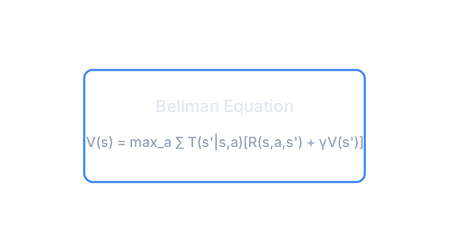
The Bellman equations supply it. They define value recursively as immediate reward plus discounted next value, which converts an infinite horizon problem into repeated one step backups. This page states both forms, expectation and optimality, and works one backup by hand. The objects being defined are covered in value functions, the iterative solver in value iteration, and the planning family that applies these backups with a known model in dynamic programming.

You need one idea first. An expectation averages over randomness. Rewards, transitions, and stochastic policies all vary, so every Bellman equation below averages over the next reward and next state rather than assuming a fixed outcome.

Think of It Like This

Resale prices on a street of houses

Each house on a street has a resale price, but no one appraises the whole street at once. An appraiser prices one house as its rental income this year plus a discounted guess at the neighbor's price next year, since buyers care about both.

Once every house carries a penciled price, the appraiser revisits each one using the updated neighbors, and the numbers settle after several passes. No one ever traces every future sale to the end of time.

Where the analogy stops: house prices reflect negotiation and taste, while Bellman values follow exact transition probabilities and a fixed discount. And the appraiser's max over buyers becomes, in control, a max over actions at each state.

How It Actually Works

Let $s$ be a state, $a$ an action, $R_{t+1}$ the next reward, $s'$ the next state, and $\gamma$ in $[0, 1]$ the discount factor. Let $V^\pi(s)$ be the expected return from $s$ under policy $\pi$ , and $V^*(s)$ the value under an optimal policy. Let $P(s' \mid s, a)$ be the transition probability. The expectation $\mathbb{E}$ averages over the randomness in $R_{t+1}$ and $s'$ .

Expectation and optimality forms

For a fixed policy the value satisfies the Bellman expectation equation:

$V^\pi(s) = \sum_a \pi(a \mid s) \sum_{s'} P(s' \mid s, a) \, \mathbb{E}[R_{t+1} + \gamma V^\pi(s') \mid s, a, s']$

In words: average over the actions the policy takes, then over where the world lands, of immediate reward plus discounted next value. For the optimal policy the average over actions becomes a max, giving Bellman optimality:

$V^*(s) = \max_a \sum_{s'} P(s' \mid s, a) \, \mathbb{E}[R_{t+1} + \gamma V^*(s') \mid s, a, s']$

The same pair exists for action values $Q(s, a)$ , which is what Q-learning updates sample. Two properties matter in practice. The backup is a contraction in the max norm with factor $\gamma$ , so repeated backups converge to a unique fixed point when $\gamma$ is below 1. And the max form is nonlinear, which is why optimal values need iterative methods rather than one linear solve at scale.

Worked example

One state, two actions, deterministic transitions, $\gamma = 0.9$ . Current estimates of the next values are $V(s'_A) = 10.0$ and $V(s'_B) = 12.0$ .

Action A pays $R = 4.0$ then lands where value is $10.0$ : $4.0 + 0.9 \times 10.0 = 4.0 + 9.0 = 13.0$ .
Action B pays $R = 1.0$ then lands where value is $12.0$ : $1.0 + 0.9 \times 12.0 = 1.0 + 10.8 = 11.8$ .
Bellman optimality keeps the max: $V^*(s) = \max(13.0, 11.8) = 13.0$ .

Action B leads to the better neighborhood but its toll is too high, so A wins this backup. On the next sweep the neighbors themselves will have fresher values and the backup repeats. The diagram draws these two candidate bars and the winning 13.0.

Code

The snippet performs the same backup and selects the maximizing action.

1def backup(reward: float, next_value: float, gamma: float = 0.9) -> float:2    """One Bellman backup: immediate reward plus discounted next value."""3    return reward + gamma * next_value4
5
6if __name__ == "__main__":7    a_value = backup(4.0, 10.0, gamma=0.9)8    b_value = backup(1.0, 12.0, gamma=0.9)9    print(round(a_value, 2))10    print(round(b_value, 2))11    print(round(max(a_value, b_value), 2))

1# -> expected output:213.0311.8413.0

Watch Out For

Pushing gamma to 0 or 1 without changing the task

The symptom: with $\gamma = 0$ the agent chases the nearest coin and ignores doors, keys, and goals one step away. With $\gamma = 1$ on a continuing task, values grow without bound and backups never settle, which looks like divergence in the optimizer.

The fix: match $\gamma$ to the task horizon, typically 0.9 to 0.99 for episodic control and strictly below 1 for continuing tasks. When behavior changes, change $\gamma$ deliberately and reexamine the learned horizon rather than retuning everything else first.

Bootstrapping from stale neighbors and calling it converged

The symptom: values stop moving after a few sweeps, but the policy is poor. Each backup averaged fresh rewards with outdated neighbor values, so the fixed point reached is for an old value landscape, not the current one. It resembles convergence while the Bellman residual is still large.

The fix: track the max Bellman residual across states, not just the policy's score, and keep sweeping until it falls below tolerance. In sample based methods the same trap appears as old target network values, which is why targets are synced on a schedule rather than frozen.

The Quick Version

The Bellman expectation equation defines a policy's value as immediate reward plus discounted next value, averaged over actions and transitions.
The optimality form replaces the action average with a max, which is the update that seeks the best policy.
Backups contract by $\gamma$ , so repeated sweeps converge to unique values when discounting is strict.
In the worked example, action A gives 13.0 and action B gives 11.8 at discount 0.9, so the backup keeps 13.0.
Residual error, not policy score, tells you when the backups have finished.